Phase Two Quant Work Summary and the Plan Ahead

Chinese

This article reviews the quant work completed in phase two, lays out the tasks of phase three, and looks ahead to phase four.

Phase Two Review

After phase one completed the implementation and warehousing of different price-volume factors, phase two naturally focused on expanding the factor library and building an ensemble modeling plus portfolio optimization framework.

Factors

Behavioral-finance factors This phase added more than ten new factors inspired by behavioral finance. In Behavioral Finance in Factor Investing, I summarized irrational expectations and irrational risk preferences on the part of investors, together with the market anomalies they create. One example is post-earnings drift: because of limited attention, investors underreact to new fundamental information, so prices do not fully incorporate it immediately and continue drifting after an earnings announcement. The same phenomenon can also be explained by sentiment and conservatism: when unexpectedly strong earnings appear, investors may remain anchored to their prior beliefs and update too slowly, leaving good news underpriced. Post-earnings drift is also significant in the A-share market and is discussed in detail in The Rationality of Irrational Finance.

Factor production routine The factor library now covers data from 2014 through the latest trading day, allowing long-horizon historical backtests. At the same time, daily bar data and tick-level data are automatically ingested for every new trading day, making factor production fully routine. Encouragingly, even though all validation and tuning were done using only data up to 2022, the factors overall have not shown obvious decay or reversal after 2023. Their consistency has held up reasonably well.

Models

Return model At the moment the strategy uses LightGBM to predict next-period return. I also surveyed advanced neural-network approaches and summarized them in Neural Networks and Cross-Sectional Asset Pricing. Broadly speaking, whether by rolling training over long historical windows, tuning GBDT hyperparameters, or designing more complex network architectures, I have not seen a meaningful improvement in final portfolio performance. Part of the reason may be that the model training objective is not well aligned with the portfolio objective. Another part is that nonlinear regularities learned entirely from in-sample data are harder to transfer out of sample when market conditions change.

Risk model The risk model took considerable effort to develop, but the final result is fairly satisfying. In the earlier article Risk Models for Alpha Strategies, I first reviewed the role of risk models and several implementation paths, including shrinkage estimation, expert-factor models, and statistical models. The final DRM-based model used in the strategy combines expert-factor and statistical-model ideas. It reuses the alpha factor library, adds market-cap and industry information, and uses a deep model to produce a set of risk factor exposures.

The role of a risk model in an alpha strategy is to predict the covariance matrix of expected returns for the underlying assets, so that portfolio variance can be minimized for a given expected return and the strategy’s Sharpe ratio can be improved. A risk model is no less important than a return model, yet compared with return modeling there is surprisingly little discussion of how to build one. One reason is that most investors simply buy commercial solutions such as Barra; another is that risk models must be judged at the portfolio level and cannot be evaluated through a simple benchmark.

Once those risk exposures are available, the next step is to estimate factor-return covariance \(\Sigma_\lambda\) and idiosyncratic volatility \(\Delta\), so that final portfolio risk can be computed:

$$ \Sigma = \Beta^T \Sigma_\lambda \Beta + \Delta $$

Here \(\Sigma_\lambda\) requires time-decay weighting, eigenvalue adjustment, and volatility-regime adjustment, while \(\Delta\) requires time-decay weighting, Bayesian shrinkage, and volatility-regime adjustment. These steps and their empirical effects are also described in Portfolio Optimization for Long-Only Multi-Factor Equity Strategies.

Portfolio Optimization

After the model layer outputs forecasts, portfolio optimization combines expected return, covariance, and turnover penalty to generate final weights. The constraint set also includes weight limits and factor-exposure bounds. In terms of speed, using the Mosek solver improved performance by about two times relative to the best open-source option.

$$ \begin{aligned} {maximize} \quad & w^T \mu - \gamma \left(f^T \Sigma_{\lambda} f + w^TDw \right) - c^T |w - w_0| \\ {subject \enspace to} & \quad {\bf 1}^T w = 1\\ & \quad 0 \le w \le w_{max} \\ & \quad f = \beta^Tw \\ & \quad |f| \le f_{max} \\ \end{aligned} $$

Here \(\mu\) is the next-day expected return forecast from the return model. The second term is portfolio risk after factor-model decomposition, and \(\gamma\) is the risk-aversion coefficient. A more detailed discussion can be found in Risk Models for Alpha Strategies. Because there are thousands of candidate stocks, the covariance matrix can easily reach tens of millions of entries. Factor models greatly simplify both estimation and computation. The final term is a linear turnover penalty, where c is estimated by a transaction-cost model or set as a hyperparameter, and can also be replaced by a quadratic penalty.

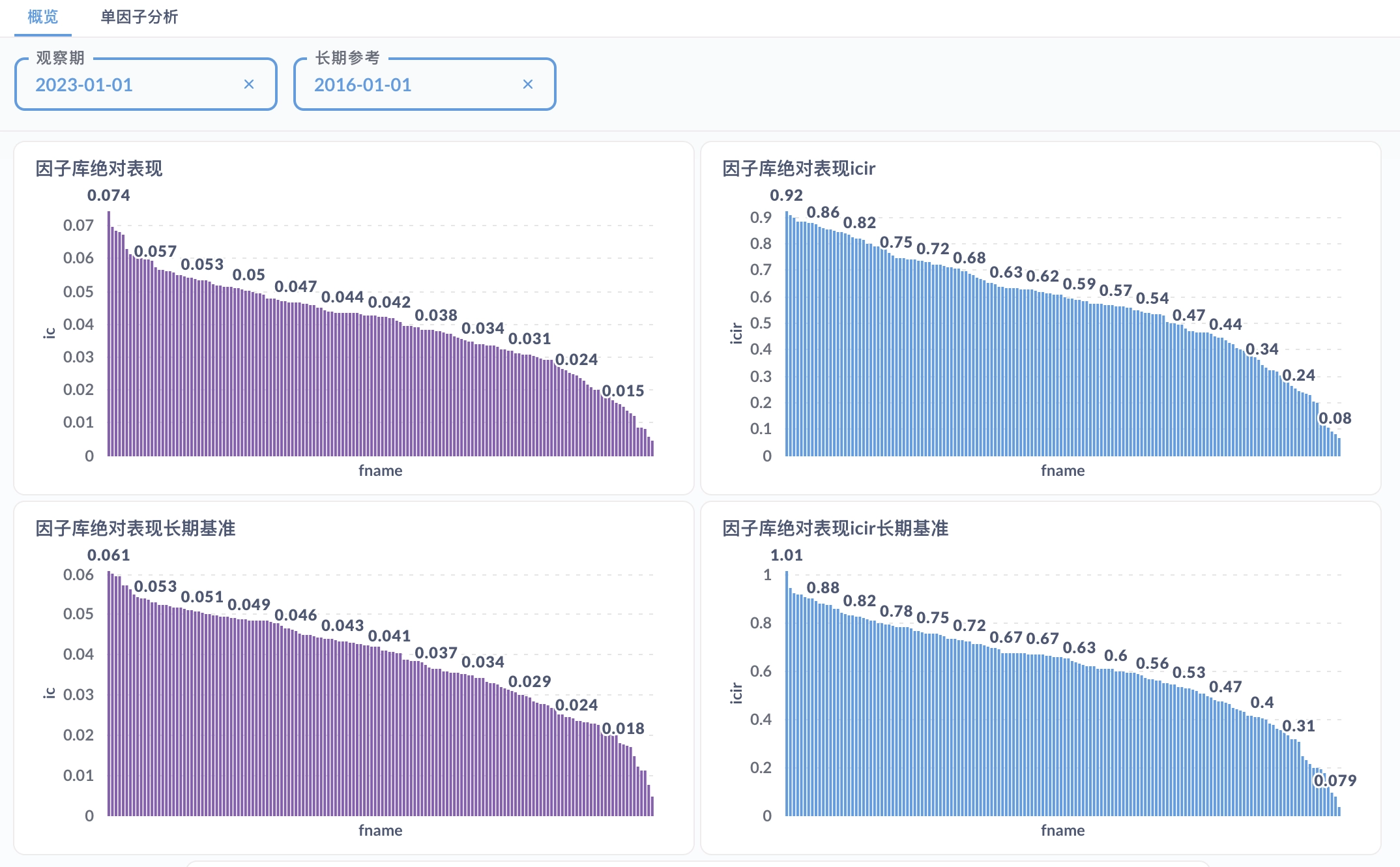
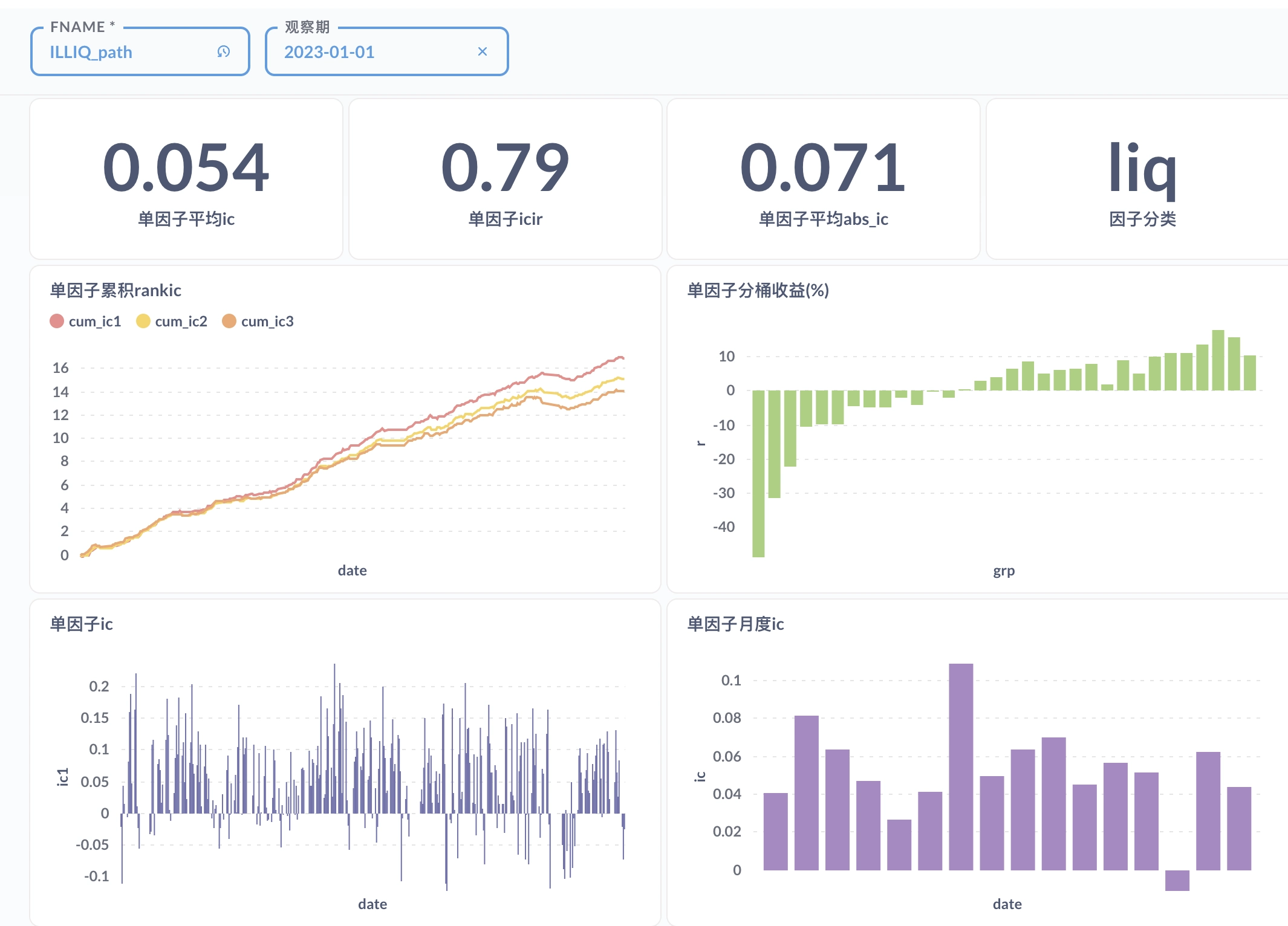
Visualization, Analysis, and Evaluation

At the factor level, I built a factor visualization and analysis platform on duckdb plus Metabase, providing both library-level and single-factor reports. Model-layer outputs will be added to the platform later.

At the portfolio level, the open-source project QuantStat is used for performance analysis. The most important evaluation metrics are discussed in Portfolio Evaluation Metrics, for example the Sharpe ratio:

$$ SR=\frac{E\left[R-R_{b}\right]}{\sqrt{\operatorname{var}\left[R-R_{b}\right]}}, $$

Phase Three Plan

The rise or fall of the empire depends on this one move.

The core of phase three is to run the strategy in live markets. It is the decisive stage, because for a high-turnover strategy, actual trading cost determines whether theoretical return can be converted into realized return.

Programmatic Trading

From an engineering perspective, the first task is fully automated trading. Programmatic trading is already standard in overseas markets and domestic futures, but it is still not widely adopted in the A-share market. Many retail investors do not even know what channels can support it, which is one reason I believe the strategy can still build an edge. The current solution is a Windows virtual machine plus miniqmt as the trading interface. The trading module, Mars, runs on Windows and communicates with the rest of the system through shared files while using the same database.

Inputs

• orders to be executed
• execution model
• factor library
• model-layer forecasts

Outputs

• account information
• trading logs
• market data

Optimal Execution for Multiple Orders

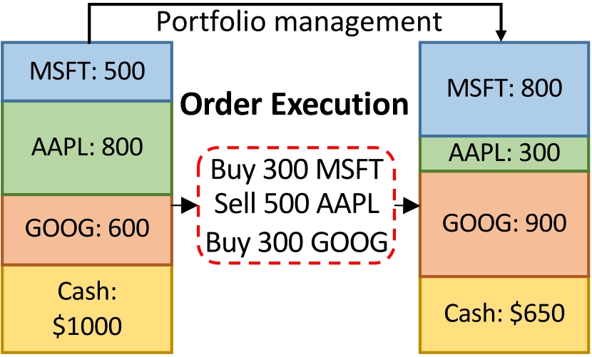
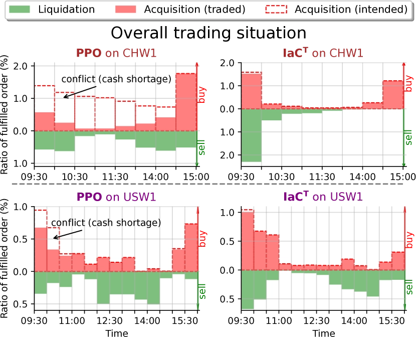
In quantitative finance, the investor’s primary objective is to maximize long-term value through continuous trading across multiple assets. This process has two parts: portfolio management dynamically allocates weights, and the execution layer aims to complete a specified set of buy or liquidation orders within a finite time window while closing the investment loop. The figure below shows the trading process during a day. The trader first updates the target portfolio under some portfolio-management strategy. Then the orders inside the red dotted box must be executed to bring the actual portfolio in line with the target. The goal is to execute multiple orders within a fixed horizon while maximizing total profit gain.

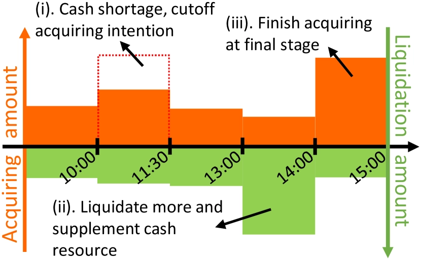
The difficulty of multi-order execution has two sides. First, the number of orders changes with daily portfolio rebalancing, so the execution strategy must scale and remain flexible. Second, cash is limited. Buy orders consume cash and only sell orders replenish it. A lack of cash may cause good opportunities to be missed, so the system must balance buying and selling to avoid conflicting decisions that create cash shortages and poor execution. The figure below shows a typical failure mode: buy orders are delayed until sell orders free up cash, causing the strategy to miss the best purchase window.

In KDD 2023, a Microsoft paper modeled the problem as multi-agent cooperation to achieve scalability and global optimality. The paper used an intent-aware communication mechanism to improve cooperative efficiency in multi-order execution.

Although the paper reports strong results, no source code is available, so it is impossible to know whether MARL is actually necessary or partly a marketing angle. My own view is that the problem could be modeled more simply as single-agent reinforcement learning. Attention mechanisms can still be used to trade off among multiple orders. The main drawback is that training imposes an upper bound on how many orders the model can handle at once, but for a small-capacity strategy that may be enough. Concretely, in an actor-critic setup, the Actor could output an N × K action tensor where N is the number of orders and K is the number of action types, while the Critic outputs one scalar value estimate.

Model and Portfolio Optimization Upgrades

Market-level information Add time, holiday, and related market-level signals to the model layer.

Feasibility filtering Filter out untradeable stocks before the optimization stage.

Transaction cost forecasting At present the portfolio optimizer uses only a simple linear turnover penalty. Once actual transaction-cost data is accumulated, the next step is to build a transaction-cost model and incorporate more granular cost estimates into weight generation.

Phase Four Outlook

After phase three, all necessary core functions should be in place. In phase four, the A-share alpha strategy will move into maintenance mode. The main task will be to improve strategic differentiation, mining alternative factors at the factor layer and introducing high-frequency models at the model layer.

Alternative Factor Mining

As the market becomes more crowded and strategies more homogeneous, many factors fail or even reverse in extreme market conditions, causing sharp net-value swings. The plan for phase four is therefore to mine alternative factors built on new data and new algorithms, with two initial priorities: relational momentum and text analysis.

Relational momentum The idea that similar stocks influence each other’s future performance is mainly grounded in three mechanisms:

• investors expect similar stocks to behave similarly, so they use the past return of one stock to infer the future return of another similar stock;
• if a stock has already performed well and an investor missed it, that investor may turn to similar stocks that have not yet moved as much, increasing demand for stocks similar to prior winners;
• if investors have made money in one stock category, path dependence makes them keep searching for similar stocks afterward.

In the earlier article Odd and Proper: A Roadmap for Alternative Factor Mining, I designed a unified KNN-based framework for relational momentum factors. In phase four, the plan is to instantiate that framework with many kinds of relationships, such as:

• industry or concept sectors
• directly computed adjacency matrices
  • mutual fund holdings
  • shared analyst coverage
  • institutional survey overlap
  • shared northbound ownership
• embedding-based distance definitions
  • historical return series
  • low-dimensional fundamental factors
  • money-flow features
  • revenue similarity
  • patent data
  • stock-name and stock-code similarity

Text analysis LLMs have been improving at high speed in recent years, and I expect to begin text-factor research in phase four using open-source models, taking advantage of technological catch-up. There are two main directions: sentiment analysis of analyst reports, which represent professional investors, and sentiment analysis of forum discussions, which represent retail investors. Analyst-report analysis is essentially about finding stocks preferred by informed investors and identifying latent value. Conversely, retail attention can be modeled as a noise-investor signal, for example by building negative factors from forum heat and emotional intensity. Many papers and reports already analyze forum sentiment, but most follow the old path of sentiment classification and fail to generate impressive portfolio results. I believe there is substantial room for improvement here. The emotions of noise traders are strongly influenced by the current tape and only weakly related to expected return, so the modeling approach should be reconsidered from the ground up. In addition, disagreement in investor expression is a natural measure of heterogeneous beliefs and can be useful for volatility prediction.

High-Frequency Models

Under the current framework, intraday high-frequency data is processed manually and downsampled to daily frequency, and the model layer trains and predicts at the daily level. After phase three is complete, I expect to obtain real-time data at the second level and derive a set of minute-level or second-level features. On that basis, the plan is to develop either neural-network time-series models or GBDT-based frequency-domain models, and then fuse or ensemble them with the existing daily model.