Neural Networks and Cross-Sectional Asset Pricing: The Art of Priors

Chinese

This article discusses how to design deep-learning models for empirical cross-sectional asset pricing by combining them with financial priors, focusing on prediction-target design, market-environment modeling, and network-architecture choices.

Introduction

The “no free lunch” theorem is a basic principle of machine learning: without reference to a specific problem, it makes no sense to debate which learning algorithm is better, because all algorithms can be regarded as equivalent in capability on average. From a Bayesian perspective, some algorithms perform better on specific problems because their built-in assumptions fit the real setting more closely. Different model structures, training methods, and loss functions can all be seen as human-injected prior knowledge. Once combined with real data samples through training, they produce posterior beliefs. Given the data, final model performance depends heavily on whether the priors are correct and whether they are expressed appropriately in the modeling process. In that sense, machine learning is the art of priors. A classic example is CNNs, whose prior of translation invariance transformed computer vision.

In quantitative investing, GBDT-style algorithms such as XGBoost and LightGBM perform extremely well on medium-scale, noisy problems like stock-return prediction. They are robust, and simply stacking a few neural-network layers usually cannot compete. So why use deep learning for cross-sectional return prediction at all? The answer is still priors. Tree ensembles cannot directly model the spatiotemporal structure of the stock market, or capture factor momentum and market sentiment. The flexibility of neural-network architectures lets us build those objects into the model and complement GBDT. The table below summarizes the links among financial theory, modeling targets, and network structures, which the rest of the article expands on.

Financial theory	Modeling target	Network structure
Multi-factor theory	prediction target	Loss
Factor momentum, market sentiment	market environment	Gating / extra feature
Inefficient-market hypothesis	temporal information	RNN / LSTM / GRU / Attention
Inter-firm links	spatial information	GCN / GAT / Hyper Graph / Attention

Prediction Targets

Training a neural network is carried out through backpropagation of the loss gradient, so the definition of the loss function directly determines the model’s prediction target and hidden assumptions. Mean squared error assumes Gaussian errors and is the standard loss for regression, so it is often used for cross-sectional return prediction. But on closer inspection, using MSE to learn the expected return of an individual asset does not fit factor-pricing theory very well. First, in both pricing theory and factor-investing practice we do not care about absolute asset performance. We care about relative performance and only need to identify the best assets relative to others, without forecasting the overall market direction. Second, even if labels are changed into relative returns, the time-varying nature of markets still makes a single common Gaussian assumption problematic.

The loss of a return model should therefore borrow from learning-to-rank. Each period can be treated as a query and the candidate assets as documents, so that a list-wise loss such as the information coefficient can be constructed. I also want to mention CCC Loss here, which simultaneously considers cross-sectional correlation and individual errors:

$$ CCCL_{x,y} = 1- \frac{2\sigma_{xy}}{\sigma^2_x+\sigma^2_y+(\mu_x-\mu_y)^2} $$

It has the equivalent form

$$ CCCL_{x,y} = 1-\frac{2\sigma_{xy}}{2\sigma_{xy}+MSE_{x.y}} $$

CCC was originally used in affective computing to measure consistency between true and predicted emotional dimensions. If predictions are shifted, the score is penalized accordingly. That is why CCC evaluates dimensional speech-emotion recognition more reliably than Pearson correlation, MAE, or MSE. Its equivalent form shows clearly that it combines cross-sectional correlation with MSE.

Return prediction contains both direction and magnitude. If magnitude is ignored and only variation is modeled, the problem becomes a risk model. In practice we often want a stable risk model defined by a set of orthogonal risk factors \(\mathbf{F}\). In 2021 Microsoft proposed DRM, the Deep Risk Model, whose goal is to obtain a risk model directly through supervised learning by carefully designing the loss. Its loss function is

$$ \min _{\theta} \frac{1}{T} \sum_{t=1}^{T}\left[\frac{1}{H} \sum_{h=1}^{H} \frac{\left\|\mathbf{y} \cdot, \mathbf{t}+\mathbf{h}-\mathbf{F}_{\cdot t}\left(\mathbf{F}_{\cdot t}^{\top} \mathbf{F}_{\cdot t}\right)^{-1} \mathbf{F}_{\cdot t}^{\top} \mathbf{y} \cdot \mathbf{t}\right\|_{2}^{2}}{\left\|\mathbf{y}_{\cdot, \mathbf{t}+\mathbf{h}}\right\|_{2}^{2}}+\lambda \operatorname{tr}\left(\left(\mathbf{F}_{\cdot t}^{\top} \mathbf{F}_{\cdot t}\right)^{-1}\right)\right] $$

The first term maximizes empirical \(R^2\):

$$ R_{\cdot t}^{2}=1-\frac{\left\|\mathrm{y} \cdot t-\mathbf{F}_{\cdot t}\left(\mathbf{F}_{\cdot t}^{\top} \mathbf{F} \cdot t\right)^{-1} \mathbf{F}_{\cdot t}^{\top} \mathbf{y} \cdot t\right\|_{2}^{2}}{\|\mathbf{y} \cdot t\|_{2}^{2}} $$

To avoid mining a large number of highly similar factors, the authors constrain the variance inflation factor so that the factors remain as orthogonal as possible. After derivation they obtain the equivalent form below, which becomes the second term:

$$ \Sigma \text{}{VIF}_i = N \cdot tr((F^TF)^{-1}) $$

Finally, the problem is defined as multi-objective optimization of explanatory power over the next N days, which gives the style factors very high autocorrelation.

This shows that by designing the loss function we can restore the original meaning of multi-factor pricing theory within a supervised-learning framework, learn differences in asset returns across the cross section, and ultimately generate both return models and risk models.

Market Environment

Existing research shows that investor optimism and pessimism under different market environments can change factor performance. For example, “defensive” factors such as low volatility usually perform better in bear markets. In addition, factor momentum is significant across global markets, meaning factor performance itself is autocorrelated. These two forms of global information cannot be introduced well through purely point-wise features and therefore call for explicit model structure.

In practice, the simplest treatment is to vectorize the global information and concatenate it with the asset feature vector as a weak feature. This was shown to work in the Jiukun Kaggle competition.

$$ x' = m \sqcap x $$

Another natural idea is to use a gating mechanism to adjust factor weights:

$$ x' = g(m) \odot x $$

Market information can also be introduced into mixture-of-experts routing or into the query of an attention mechanism. In principle, a data-driven sense of the market environment should help the model perform better across full cycles, though it also imposes higher demands on data scale and regularization.

Spatiotemporal Structure

At the model level, GBDT treats all samples equally and does not consider links among assets, that is, it ignores spatial structure. Yet finance theory suggests that markets exhibit “momentum spillover”, where related firms show lead-lag relationships in returns. This linkage stems from investors’ limited attention: information is not instantly reflected across similar firms, but diffuses over time. The table below lists several known types of such relations.

Literature	Effect
Hou (2007)	intra-industry effect
Cohen and Frazzini (2008)	supplier-customer effect
Cohen and Lou (2012)	conglomerate lead-lag effect
Lee et al. (2019)	technological links
Parsons, Sabatucci and Titman (2020)	geographic lead-lag effect
Ali and Hirshleifer (2020)	shared analyst coverage

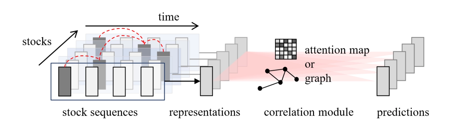
From the perspective of deep-learning architecture, graph neural networks are well suited to this kind of relationship: companies are nodes, relationships are edges or hyperedges, and features from similar stocks are aggregated.

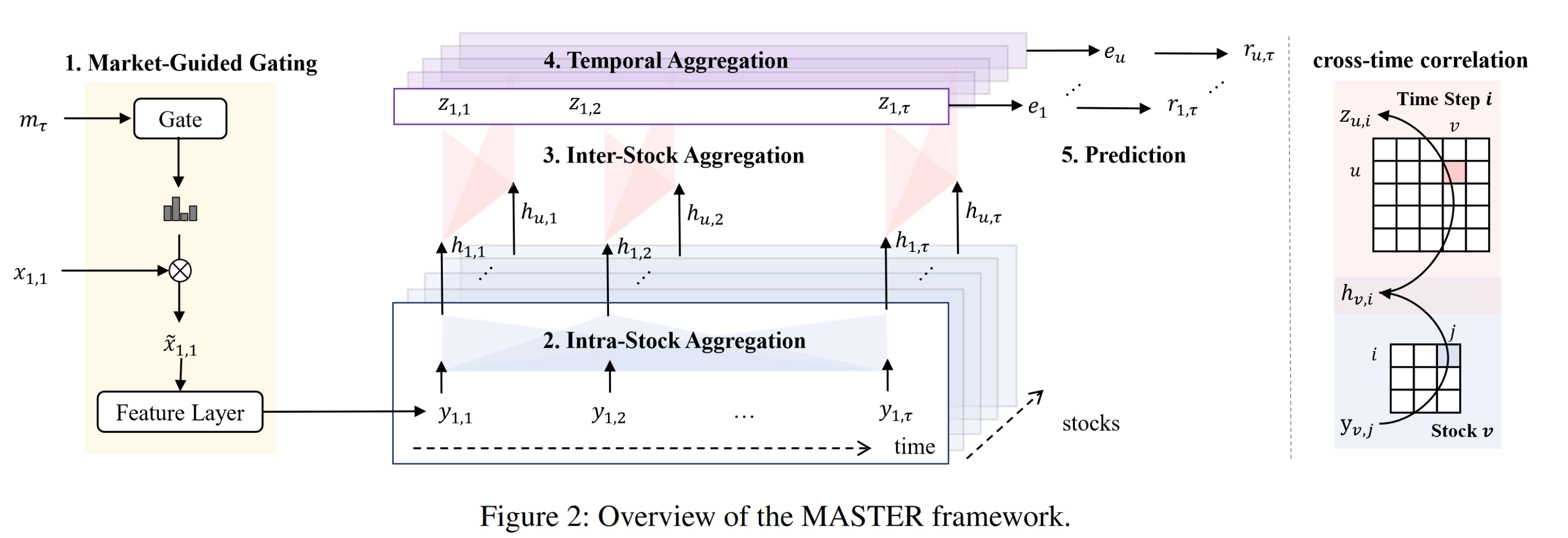
Because the number of stocks in a cross section is not that large, it is also feasible to use multi-head self-attention, the core module of Transformers, to compute the full set of relations directly. In that case, links among stocks are driven entirely by data without manual definition. The relational information can be injected through features and modeled implicitly. For example, the AAAI 2024 MASTER network uses attention to model both time and space.

On the time dimension, modeling sequences of asset feature vectors can also improve prediction. Most existing work uses a three-stage structure: temporal-information extraction, spatial modeling, and final prediction. Mature and common architectures for extracting temporal information include recurrent networks such as LSTM and GRU, as well as attention mechanisms.

Conclusion

My view is that purely data-driven methods cannot succeed in asset pricing. Any effective model should combine specific human priors with data. Researchers should start more from financial priors and free deep-learning models from the alchemy-like trap of blindly tuning them.