Algorithmic Trading Strategies Based on Deep Reinforcement Learning
There is broad market demand for algorithmic trading. This article analyzes how to implement algorithmic trading from the perspective of deep reinforcement learning, including policy inputs and outputs, reward functions, and neural-network structure. Compared with traditional methods, DRL has clear advantages in optimal execution across multiple orders and does not require precise mathematical modeling of time-varying market microstructure. The policy is optimized toward a global objective. Finally, the article also considers how intraday trading strategies can be integrated organically with alpha strategies.
Algorithmic Trading
Whether a trade originates from a discretionary human decision or from a quantitative system’s instruction, it still needs a concrete execution process before it becomes the target position. Using an algorithmic trading strategy to place orders and optimize transaction cost is highly beneficial for final investment performance and is already standard market practice. In stock multi-factor strategies, for example, it is common to assume execution at the next trading day’s volume-weighted average price plus transaction cost, such as 2 per mille, and to use that as the prediction target for the return model. Under different realized transaction costs, the performance of an alpha strategy can diverge dramatically, especially for relatively high-turnover daily strategies.
The first generation of algorithmic trading strategies was almost passive. TWAP, the time-weighted average price algorithm, is the simplest traditional execution strategy and suits relatively liquid markets and modest order sizes. It divides the trading interval uniformly and submits equally sized slices at each subdivision point.
$$ \text{TWAP}=\frac{\sum_{t=1}^N{p_t}}{N} $$
The VWAP algorithm introduces a prediction of volume distribution. The usual implementation divides the trading day into several time intervals, fits the share of volume in each interval from historical data, and then executes in proportion to those predicted volume shares so that realized cost stays close to VWAP.
$$ \text{VWAP}=\frac{\sum_{t=1}^N{amount_t}}{\sum_{t=1}^N{volume_t}} $$
The second generation of trading algorithms brought opportunity cost and execution risk into the framework. These methods focus on impact cost and use increasingly refined models of random price movement in order to achieve better execution than TWAP or VWAP. Representative examples include implementation shortfall and arrival-price strategies.
But this class of execution algorithm, built on explicit modeling of market microstructure, is inherently suboptimal. Take stock multi-factor strategies as an example: if execution timing is unconstrained, the whole trading day is feasible. In theory, one would need to model the full-day price path and volume distribution of each stock in order to derive the optimal order schedule that beats the day’s VWAP, not to mention solving the multi-order optimal-execution problem at the same time. That level of explicit modeling is simply beyond human analytical capacity. A data-driven method can instead bypass direct market modeling altogether: feed in market information and let the model produce the trading decision directly. The large amount of high-frequency intraday price-volume data makes this end-to-end approach feasible.
An analogy can be made to Go AI. Early Go engines relied heavily on heuristic rules defined by experts, such as protecting corners or building eyes. Those rules came from human experience and theory, and the resulting programs only barely approached professional strength. AlphaGo, by contrast, used deep reinforcement learning as its core and followed a fully end-to-end route. The neural network only estimated the winning probabilities of candidate moves and improved policy through self-play. The strategic reasoning behind the moves became opaque, but the style was imaginative, proactive, and overwhelmingly superior to the best human players. The algorithmic trading strategy discussed in this article takes the same DRL-centered approach, which is also the newest direction in the academic literature.
A Reinforcement-Learning Perspective
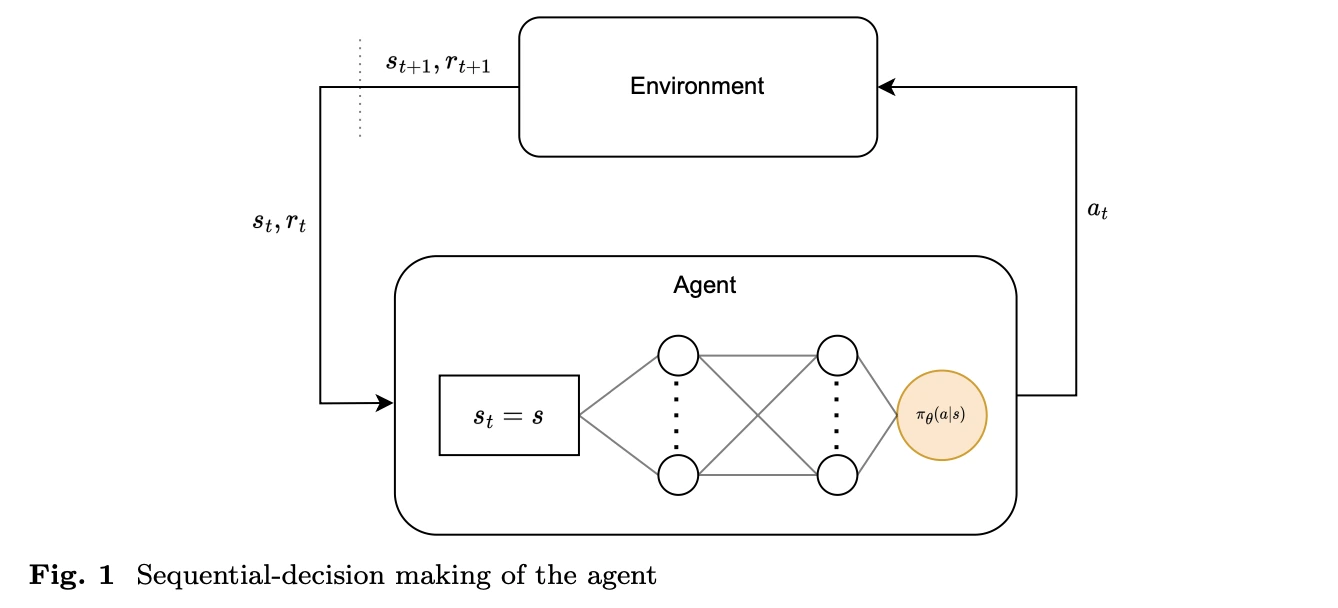
A Markov decision process is the basic framework of reinforcement learning and is used to describe sequential decision problems. An MDP is usually defined by four core elements: state (S), action (A), state-transition probability (P), and reward (R). For long-term decisions, a discount rate (\(\gamma\)) is often added, forming the five-tuple (S, A, P, R, \(\gamma\)) that describes the system’s dynamics and decision process. In reinforcement learning, the agent interacts repeatedly with the environment and learns what state transitions and rewards follow from taking a given action in a given state. This learning process based on states, actions, and rewards is why the MDP is the central theoretical tool of reinforcement learning.
An intraday trading strategy is exactly a sequential decision problem that repeatedly processes the latest market information. At each point in time, the strategy needs to make buy or sell decisions based on real-time market information in order to achieve the best trading outcome. That matches the assumptions of the MDP almost perfectly, because in intraday trading the trader, or agent, selects an action (A) based on the current market state and account state (S), observes the market response (P), and receives a corresponding reward (R). This approach can handle complex market dynamics while continuously iterating the policy to adapt to changing conditions.
State Space
Unlike many standard reinforcement-learning tasks, where the agent’s actions directly affect its own state, in smaller-scale trading strategies the observed state naturally splits into public information that is not affected by the order itself, such as market movements, and private information that changes directly, such as cash balance and position. That means the market-encoding module can be separated from the rest of the model during training and deployment and trained or inferred on its own. The specific components of the state space are discussed below.
Basic price-volume information Open, high, low, and latest prices are the basic price inputs, while amount and volume are the basic trading inputs. Derived features include returns and interval volume.
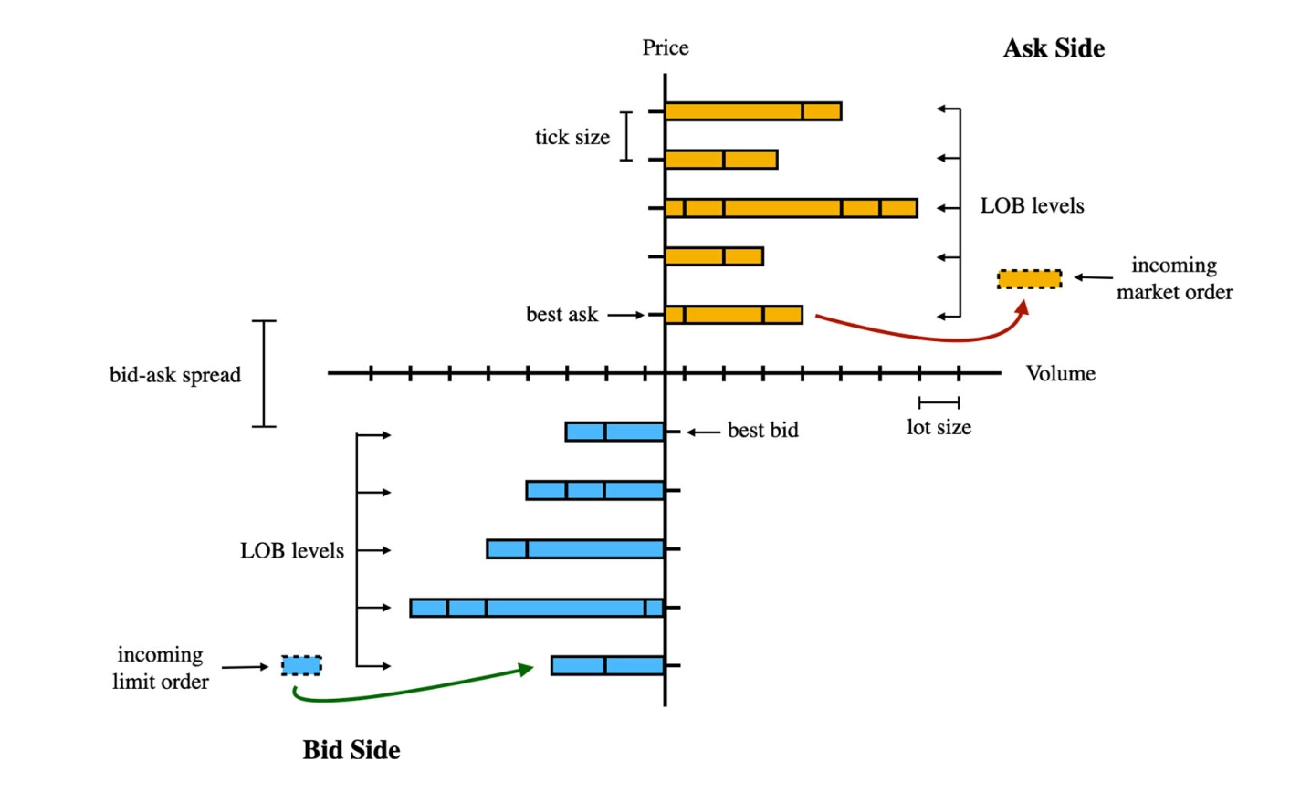
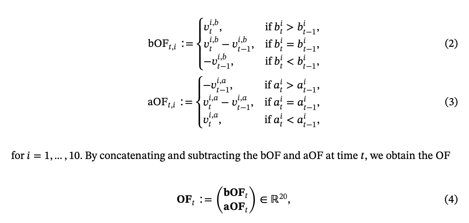
Limit order book Market microstructure is a key part of relatively high-frequency intraday algorithms. The limit order book is the real-time record of buy and sell orders submitted at specific prices by market participants. It shows intent and size at each price level and therefore reflects supply and demand. The order book provides a real-time snapshot of market demand and supply that helps investors understand market conditions. To extract features directly from the book, one can compute indicators such as the spread and the micro-price. Transforming the order book into non-stationary order flow is also a common preprocessing method.

Daily-frequency features Beyond intraday prices and microstructure, adding alpha factors can inject longer-horizon incremental information at daily or weekly frequency into the intraday strategy. In practice this helps the model understand stock characteristics and forecast return distributions.
Private information An execution algorithm necessarily serves a specific account, so it also needs the current position, available cash balance, and remaining trading task as inputs.
Action Space
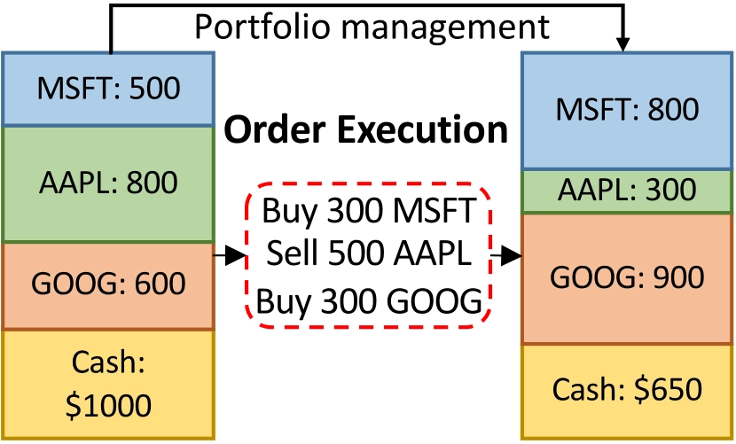
In reality, order placement has a great deal of freedom, but the action space in DRL needs careful design. A trader can choose market orders, limit orders, best-five-level orders, and so on, while order direction and size can also be fully customized. If the program is allowed to place orders freely on both sides without quantity constraints, it could in theory learn a high-frequency market-making strategy. But too much freedom also makes the model hard to train, weakens generalization, and makes it difficult for the simulation environment to reproduce the market accurately. Regulation also places limits on intraday reverse trading. For these reasons, I think it is necessary to reduce the degrees of freedom in the action space by fixing direction, execution price type, or order size. In Microsoft’s KDD 2023 paper, for example, the action for a given execution task is to submit one portion of the order at market each time, with \(a_t^i \in \left{ 0,0.25,0.5,0.75,1 \right}\), and reverse trading is not allowed. That design is reasonable when the algorithm serves portfolio rebalancing. If the target is instead to overlay an intraday T0 strategy on top of an alpha strategy, the direction constraint can be relaxed and the base position can be used for intraday trading. An additional benefit of this intraday strategy is that end-of-day holdings still match the intended portfolio, which makes performance attribution much easier.
Reward Function and Simulation Environment
For a trading algorithm, short-term return is not the main point. What matters is a broader global view. In reward design, the first objective is to capture how well the algorithm optimizes transaction cost through timing:
$$ R_e(s_t,a_t^i;i) = d_i a_t^i (\frac{p_t^i}{\tilde{p^i}}-1) $$
The second is to account for impact cost, for example through a quadratic function:
$$ R^-(s_t,a_t^i;i) = -\alpha (a_t^i)^2 $$
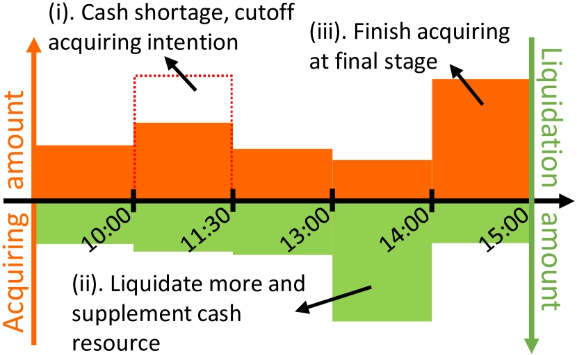
Finally, the policy should be penalized when cash runs out, because insufficient cash creates opportunity cost when buy orders cannot be executed. The model should learn to exchange for cash earlier rather than wait only for the best sale price.
$$ R_c(s_t,a_t^i;i) = -\beta \mathbb{I}(c_t=0|c_{t-1}>0) $$
During training, feedback comes from an offline simulation environment because the cost of online training is unacceptable. That places high demands on simulator performance, so my plan is to implement the environment in Cython. The simulator also needs to model order-fill probability and execution ratio.
Deep Policy Network
The action policy in DRL is a standard neural network, \(\pi(a_t^i|s_t)\).
Market Encoding and Auxiliary Tasks
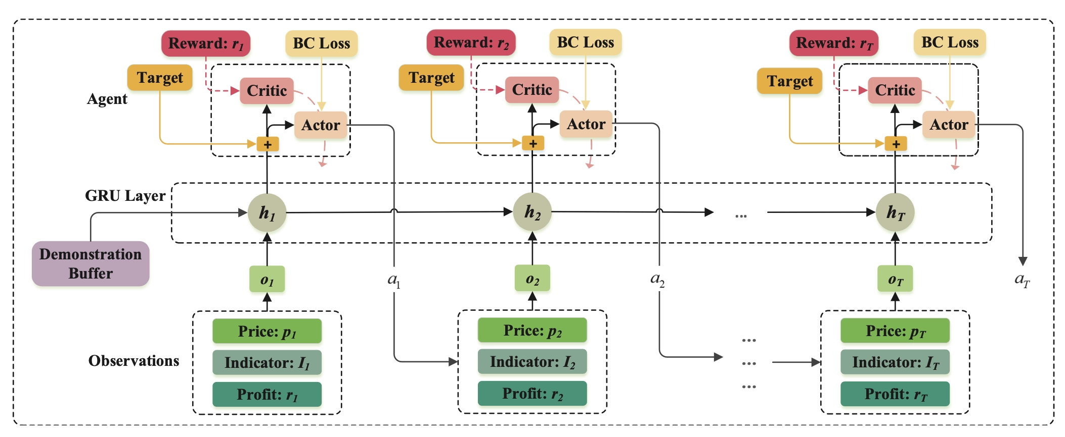
As noted earlier, the public information in the state is independent of the agent’s action, so it can be encoded with a separate module and stored as embeddings for RL training. The benefit of this two-stage setup is that it improves training efficiency and avoids policy instability caused by end-to-end training. How should the pretraining labels be constructed? The simplest idea is to use an autoencoder to preserve all original information. But if future returns and future volume distribution are known, the policy can make globally optimal decisions, so future distribution information can also be used as a label. My plan is to combine both ideas. The latter is similar to introducing risk-aware or return-aware auxiliary tasks into an end-to-end objective.
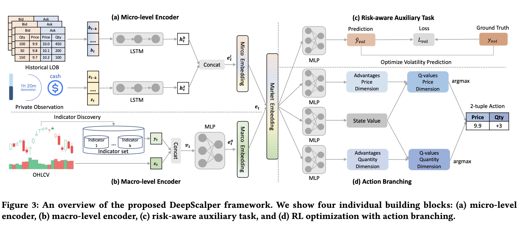
In terms of network architecture, because feature engineering is intentionally kept simple for deployment reasons, the encoder should use structures that aggregate temporal information, such as LSTM or GRU.
The figures below show two feasible overall model structures.
The Multi-Order Execution Problem
How can multiple-order execution be modeled explicitly so that insufficient liquidity can be avoided?
One answer is to define multi-order tasks as the basic simulation unit during training and search for the global optimum within each simulation. Another is to introduce attention mechanisms in the network architecture so that global information can inform actions on a single stock.
Extensions
In breadth, DRL-based trading algorithms can be applied across stocks, futures, cryptocurrencies, and other markets. In depth, the methods described here can be used purely to execute rebalancing tasks, or as a T0 overlay on a base portfolio, or even independently as a high-frequency arbitrage strategy.
One point worth noting is that when an intraday strategy is overlaid on an existing alpha strategy, the profits or costs generated by trading different stocks should be taken into account. The portfolio-optimization objective can then be written as
$$ \max_w \quad w^T (\mu+\kappa) - \gamma w^T \tilde{\Sigma} w - c |w - w_0| $$
where \(\mu\) is the expected return vector, \(\tilde{\Sigma}\) is the estimated covariance matrix, and \(c\) is a constant that represents rebalancing cost. \(\kappa \in \mathbb{R}_+^ {N}\) is the profit contribution from holding different stocks as the base position: in each period there are two trading opportunities, one in each direction, and the difference from VWAP is the profit that can be generated. Since the third term already penalizes turnover, \(\kappa\) is always positive. A simple handcrafted model can be used to estimate \(\kappa\). Because real transaction-cost data can only be obtained through actual trading with real money, model complexity should be kept as low as possible, and the model parameters themselves will become an important asset for the strategy developer.
Algorithmic Trading Strategies Based on Deep Reinforcement Learning