Convertible Bond Quant Strategy: Alpha Selection, CCB Pricing, and Futures Hedging

Chinese

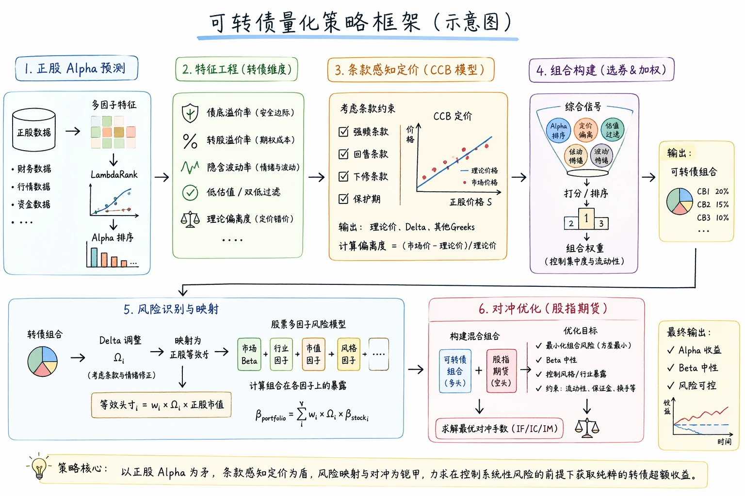
As traditional dual-low strategies gradually lose their effectiveness, what else can be done in convertible bond investing? This article introduces a complete quantitative framework for convertible bonds: using equity multi-factor Alpha to drive security selection, using the CCB pricing model as the strategic hub linking returns and risk control, and finally using stock index futures to hedge Beta.

Overview

From “Low-Valuation Premium” to “Underlying-Stock Alpha Competition”

For a long time, excess returns in convertible bonds came primarily from “pricing inefficiency”: traditional dual-low strategies (low price and low premium), or low implied-volatility-spread strategies based on the BS model, could generate significant returns through high-win-rate mean reversion alone. But when we combine recent data with changes in market microstructure, this logic has fundamentally reversed.

• Systematic decline of valuation factors Since the second half of 2022, traditional low-valuation factors, especially implied volatility spread and dual-low, have deteriorated markedly in equity-like convertibles, and have even delivered negative Alpha during certain periods.
• “Cheap” means “a trap” As the market has become more institutionalized, with public-fund holdings reaching record highs, and as passive ETF capital has expanded, pricing efficiency has improved substantially. Today, “extremely low valuation” often reflects the market’s full pricing-in of deteriorating underlying-stock fundamentals rather than a mistaken sell-off. Buying “cheap” convertibles is, in essence, exchanging the tail risk of a decline in the underlying stock for limited room for valuation repair. In an environment where competition around the underlying stock is intense, the payoff is poor.

As a result, the core contradiction in convertible-bond investing is no longer simply about finding “undervalued options,” but about identifying the underlying stocks that truly have upward drivers. Low-valuation indicators have not lost all significance, but they are now better suited as tools for margin of safety and risk filtering, rather than as the sole logic for security selection. To avoid falling into the “cheap means trap” pitfall, we directly introduce Alpha forecasting for the underlying stock and use it as the primary driver of convertible-bond selection.

Cross-Asset Reuse of Alpha

Migrating Alpha forecasting capability from a mature equity multi-factor framework into a convertible-bond strategy is, in essence, treating convertibles as “stocks with built-in leverage and downward-reset protection.”

• Underlying-stock driven Research from Sinolink Securities shows that after introducing price-volume factors such as Alpha158 and fundamental factors, model explanatory power for equity-like convertibles improves significantly. We directly reuse the existing multi-factor library, covering high-frequency price-volume data, fundamental expectations, capital flows, and more, to forecast the future performance of the underlying assets behind convertible bonds.
• LambdaRank ranking Portfolio construction is fundamentally a Top-K ranking problem. We introduce the LambdaRank framework and optimize directly for NDCG (Normalized Discounted Cumulative Gain), concentrating modeling power on the ranking accuracy of the highest-scoring names, while using a nonlinear structure to handle the complex interactions between equity factors and convertible-bond terms, such as forced-redemption countdowns and reset-game dynamics.

A Closed Loop of Pricing, Risk Control, and Hedging

To deliver stable absolute returns, this strategy does not stop at pure long exposure. Instead, it builds a refined closed loop of pricing, risk control, and hedging.

• CCB pricing If a simplified pricing model ignores clause constraints such as redemption, put provisions, and protection periods, it will often produce systematic biases in both price and Delta for equity-like convertibles. The direction of the bias depends on the bond’s state, the length of the protection period, and the strength of the redemption constraint. For live risk control, it is therefore more prudent to use the CCB model, which captures the path dependence of contract terms.
• Risk-factor mapping Using the Delta computed by the CCB model, we map the risk exposure of the convertible-bond portfolio precisely into an equity multi-factor risk model.
• Futures hedging Based on risk-model attribution, the portfolio’s total exposure is decomposed into market Beta, style exposure, and industry deviation. Among these, stock index futures (IF/IC/IM) are used mainly to reduce market-direction and size-style risk, while industry-level deviations are controlled more through portfolio constraints and position optimization.

Feature Engineering

Feature engineering is the translation process that turns market data into investment views. We distill information into three dimensions: valuation protection based on asymmetry, game premiums based on microstructure, and Alpha mapping derived from underlying-stock forecasting.

Valuation and margin of safety form the defensive base of the strategy rather than an independent return engine. The bond-floor premium measures how much support the convertible has as a straight bond, and a lower bond-floor premium usually implies stronger downside protection. The conversion premium, meanwhile, reflects the transaction cost and sentiment premium embedded in option pricing. This article still retains valuation indicators such as dual-low, but uses them mainly to control margin of safety, filter out overvaluation traps, and combine them with underlying-stock Alpha signals, rather than continuing to view mean reversion as a stable and independent source of return. At the same time, we also introduce a theoretical-pricing deviation metric to identify local mispricing opportunities under contractual constraints.

Microstructure and game-related features aim to capture incremental returns arising from behavioral bias and institutional constraints. Outstanding convertible balance, that is, the size of the issue still in circulation, is a highly explanatory factor: small issues often outperform the broad market, reflecting a combination of liquidity premium and institutional neglect. Large public funds are constrained by liquidity thresholds and cannot build large positions in them, allowing nimble quantitative strategies to arbitrage where pricing efficiency is insufficient. In terms of turnover, in low-valuation regions, high turnover often signals that smart money is accumulating positions. We incorporate the combination of “low valuation + high heat” into the model to capture explosive upside during the early phase of sentiment repair. Contractual games, such as forced-redemption countdowns and willingness to reset the conversion price, are also quantified and turned into predictable event-driven signals.

Underlying-stock multi-factor mapping is the key to transferring equity Alpha. The first-order driver of price changes in convertible bonds is the fundamentals and market performance of the underlying stock. Traditional convertible-bond strategies look only at the historical performance of the stock, that is, momentum, which is essentially a rear-view-mirror-style linear extrapolation. We directly connect to a mature equity multi-factor system and use the stock-side forecasts of future excess returns (Predicted Alpha), fundamental expectation surprises, and institutional capital flows directly as feature inputs for convertibles. In this way, rather than passively waiting for a rise in the underlying stock to pull the bond higher, we position in advance in the convertibles associated with names whose fundamentals are improving and attracting major capital inflows.

Ranking Model: LambdaRank

In the special market of convertible bonds, directly forecasting absolute returns faces two challenges at once: “sample sparsity” and “distribution nonlinearity.” For this reason, the strategy introduces the LambdaRank learning-to-rank model and shifts the mathematical objective from “predicting a value” to “predicting the relative order.”

Why Abandon Regression

The small-sample trap There are more than 5,000 stocks in the full market, enough for a regression model to fit a relatively smooth mean, but there are only about 500 convertible bonds. Minimizing mean squared error on such a small sample:

$$ L = \sum_{i=1}^{N} (y_i - \hat{y}_i)^2 $$

is extremely vulnerable to noise. In order to accommodate the large number of mediocre middle-ranked samples, the model often sacrifices predictive accuracy on the top names. But in investing, we only care who ranks in the top 20, not the difference between No. 200 and No. 201.

Return-distribution mismatch Our input features contain a large number of equity factors, which are approximately normally distributed, while the target variable, convertible-bond return, exhibits a pronounced “right-skewed long-tail” structure, with losses truncated below by the bond floor and upside left open by the embedded option:

$$y_{stock} \sim N(\mu, \sigma^2) \quad \text{vs} \quad y_{cb} \sim \text{Skewed Distribution}$$

This difference in distributional shape between input and output makes it difficult for a regression model to achieve high-precision fitting through a simple functional mapping \(f(X) = Y\).

How LambdaRank Works

LambdaRank is a Pairwise gradient-boosting algorithm. Its core idea is to turn the “scoring” problem into a “horse race”: there is no need to predict the exact return of each bond, only to predict which one should rank ahead of which.

Pairwise probability For convertible bond A and convertible bond B, the model computes the probability that A is more worth buying than B:

$$P_{ij} = \frac{1}{1 + e^{-\sigma(s_i - s_j)}}$$

where \(s_i\) and \(s_j\) are the model scores assigned to the two bonds, and \(\sigma\) is a scaling parameter.

Lambda gradient If convertible bond A’s true return is higher than B’s, but the model ranks B ahead of A, the algorithm generates an upward force \(\lambda\) pushing A higher. The magnitude of that force is determined by two components: the severity of the ranking error and the importance of the position, that is, \(\Delta\text{NDCG}\). Misranking No. 1 and No. 201 creates a far larger “force” than misranking No. 200 and No. 400. Mathematically:

$$\lambda_{ij} = \frac{\partial C}{\partial s_i} = \underbrace{\frac{-\sigma}{1 + e^{\sigma(s_i - s_j)}}}_{\text{Ranking-probability gradient}} \times \underbrace{|\Delta \text{NDCG}|}_{\text{Position weight}}$$

Intuitively, the model automatically concentrates optimization on the top of the universe. Even with only 500 samples, it ignores ranking noise among the bottom 400 bonds and focuses all its effort on correctly ranking the top 50 high-return names.

Through LambdaRank, we avoid the problems of limited convertible-bond samples and skewed distributions, use NDCG to concentrate computational power on the head of the distribution that matters most for investment results, and achieve nonlinear relative-strength selection based on underlying-stock multi-factor signals. For the full derivation path from RankNet to LambdaRank to LambdaMART, and for the detailed definition of NDCG, see A Concise Introduction to Learning to Rank (LTR).

The CCB Pricing Model

In an absolute-return strategy, pricing accuracy directly determines the success or failure of hedging. If a simplified pricing model ignores the Chinese convertible-bond market’s distinctive “redemption clauses” and “redemption protection period,” it will often produce systematic biases in both the price and the Delta of equity-like convertibles. The direction of the bias depends on the strength of contractual constraints and the state of the bond, so a pricing framework that captures path dependence is required.

This strategy adopts the CCB (Callable Convertible Bond) model proposed in research by Guosheng Securities. Based on the Complete Decomposition Method, it uses the analytical solution derived by Zhou Qiyuan (2008, 2009). This method fully embeds the path-dependent features of forced redemption and put provisions, and because it has an analytical expression, it is significantly superior to binomial trees or Monte Carlo simulation in both computational efficiency and the stability of Greeks estimation.

Core Logic

Under the risk-neutral measure, the CCB model decomposes the value of the convertible bond \(V_{CCB}\) into expected equity cash flow (\(ccb_{equity}\)) and expected bond cash flow (\(ccb_{bond}\)):

$$V_{CCB} = ccb_{equity} + ccb_{bond}$$

The key to the model is the precise partitioning of future paths for a callable convertible bond with a redemption protection period. Let the end date of the redemption protection period be \(t^p\), the maturity date of the convertible bond be \(t^m\), the redemption trigger price be \(h\) (typically 130% of the conversion price), and let the path of the bond’s parity \(S_t\) be divided into four mutually exclusive cases:

• Path 1 (immediate redemption): at \(t^p\), parity \(S_{t^p} \ge h\), triggering forced redemption and ending the bond immediately.
• Path 2 (mid-term redemption): the trigger is not reached at \(t^p\), but parity touches the redemption barrier \(h\) during the period from \(t^p\) to \(t^m\).
• Path 3 (conversion at maturity): redemption is never triggered over the life of the bond, and at maturity parity \(S_{t^m} >\) bond terminal value \(fv_N\), so the investor chooses conversion.
• Path 4 (redeem as bond at maturity): redemption is never triggered over the life of the bond, and at maturity parity \(S_{t^m} \le fv_N\), so the investor holds to maturity.

Pricing Formula

The expected equity cash flow (\(ccb_{equity}\)) is contributed by the first three paths, weighting equity value by probability under different trigger conditions:

$$ccb_{equity} = \underbrace{e^{-r_f t^p} E^Q[S_{t^p} I(A_1)]}_{\text{Path 1: redeemed immediately after the protection period}} + \underbrace{h E^Q[e^{-r_f t^*} I(A_2)]}_{\text{Path 2: redemption triggered during the life of the bond}} + \underbrace{e^{-r_f t^m} E^Q[S_{t^m} I(A_3)]}_{\text{Path 3: conversion at maturity}}$$

where \(I(A_i)\) is the indicator function representing the event that path \(i\) occurs.

The expected bond cash flow (\(ccb_{bond}\)) includes deterministic coupons during the protection period, coupons after the protection period conditional on the bond not having been redeemed, and the principal repayment at maturity under Path 4:

$$ccb_{bond} = \sum_{i=1}^{n_1} pv_i + \sum_{i=n_1+1}^{N-1} pv_i \cdot p_{in}(t_i^c) + pv_N \cdot E[I(A_4)]$$

• \(pv_i\): the present value of the bond cash flow in period \(i\).
• \(p_{in}(t_i^c)\): the probability that the convertible bond has not yet been redeemed by the coupon payment date of period \(i\).
• \(E[I(A_4)]\): the probability that Path 4, holding to maturity, occurs.

Analytical solution To compute Delta in milliseconds in live trading, we use the analytical results in Zhou Qiyuan (2009) directly. Define the auxiliary variables:

• \(u = r_f - \frac{1}{2}\sigma^2\), \(\hat{u} = r_f + \frac{1}{2}\sigma^2\), \(\tilde{u} = \sqrt{u^2 + 2\sigma^2 r_f}\)
• \(K_1 = \ln(fv_N / S_0)\), \(K_2 = \ln(h / S_0)\)

The analytical expressions for each expectation term are as follows:

(1) Path 1 (redeemed immediately at the end of the protection period):

$$E^Q(S_{t^p} I(A_1)) = S_0 e^{r_f t^p} N\left( \frac{\ln(S_0/h) + \hat{u}t^p}{\sigma\sqrt{t^p}} \right)$$

(2) Path 2 (mid-term redemption):

$$E^Q(e^{-r_f t^*} I(A_2)) = \left(\frac{h}{S_0}\right)^{(u-\tilde{u})/\sigma^2} \left[ G(t^m) - G(t^p) + H(t^p, t^m) \right]$$

where \(G(\tau)\) and \(H(\tau_1, \tau_2)\) involve the bivariate normal distribution function \(N_2\), which is used to handle the distribution of the path-dependent first-passage time.

The analytical expressions for Path 3 (conversion at maturity) and Path 4 (redeem as bond at maturity) are both lengthy. Each can be written in closed form in terms of the bivariate normal distribution function \(N_2\), with their full structure jointly determined by boundary conditions, first-passage probability, and the terminal state at maturity, so the full expansion is omitted here. Economically, the former corresponds to the equity value of “no redemption triggered and conversion at maturity,” while the latter corresponds to the bond value and occurrence probability of “no redemption triggered and held to maturity.” In live trading, the analytical solution is called directly to compute price and Greeks.

Delta Adjustment and Application

Compared with simplified models that ignore contractual constraints, the CCB model is not only closer to real trading constraints in pricing, with pricing error centered near 0%, but also provides a Delta more consistent with the bond’s contractual state:

$$\Delta_{adj} = \frac{\partial V_{CCB}}{\partial S}$$

For convertible bonds close to the forced-redemption trigger, with short protection periods, or with markedly stronger contractual constraints, simplified models often struggle to capture accurately how fast Delta changes. By explicitly incorporating path dependence, the CCB model can provide more stable estimates of risk exposure for hedging and risk control, while also supplying accurate input vectors to the downstream quadratic-programming risk-control model.

Risk Control: Factor Penetration and Futures Hedging

After completing feature extraction through LambdaRank and CCB pricing, we obtain a long-only convertible-bond portfolio that is theoretically rich in Alpha potential. Convertible bonds are a hybrid of equity risk, credit risk, and volatility risk. Without refined risk control, market Beta fluctuations can easily swallow Alpha.

This section explains how to build a quadratic-programming (QP) risk-control system based on the covariance matrix, with a focus on solving the core challenge of hidden Delta exposure caused by changes in market sentiment, as reflected in conversion premiums.

Why Simple Market-Value Hedging Is Not Enough

If we simply compute the portfolio’s total notional principal, multiply it by an average Delta such as 0.6, and short stock index futures of the corresponding market value, two problems arise:

1. Style mismatch (Basis Risk): underlying names of convertible bonds generally tilt toward mid and small caps, such as CSI 1000 and Guozheng 2000, while stock index futures such as IF/IH tilt toward large caps. Simple hedging creates a style exposure of “long small caps, short large caps.”
2. Non-linearity: the Delta of convertible bonds changes dynamically. When the market sells off sharply, convertibles fall back toward their bond floor and Delta declines quickly. If futures shorts are not adjusted in time, the result is over-hedging and losses.

A multi-factor risk model must therefore be introduced to dissect the risk of the convertible-bond portfolio into factor exposures across different dimensions and strip them out precisely through mathematical optimization.

From Convertibles to Factors: Risk Penetration

Using the CCB-model-adjusted Delta (\(\Delta_{adj}\)), we map “convertible-bond holdings” into equivalent “equity holdings,” and then map those further into “risk factors.”

Basic mapping For convertible bond \(j\), let the corresponding underlying stock be \(S_j\), with price \(P_j\). The return elasticity of the convertible bond with respect to the underlying stock is:

$$\Omega_j = \Delta_{adj, j} \times \frac{S_j}{P_j}$$

This means that if the underlying stock rises 1%, the convertible bond should theoretically rise by \(\Omega_j%\). The exposure of the convertible-bond portfolio to risk factor \(k\), such as industry, size, or momentum, is:

$$\beta_{cb, k} = \sum_{j \in Portfolio} w_j \cdot \Omega_j \cdot \beta_{stock_j, k}$$

Sentiment adjustment Convertible-bond prices depend not only on the underlying stock, but also on the conversion premium, that is, implied volatility \(\sigma_{imp}\):

$$P_{cb} = f(S, \sigma_{imp}, t, \dots)$$

According to the total differential, changes in convertible-bond price come from:

$$dP = \underbrace{\frac{\partial P}{\partial S} dS}_{\text{Underlying-stock driven (Delta)}} + \underbrace{\frac{\partial P}{\partial \sigma_{imp}} d\sigma_{imp}}_{\text{Sentiment driven (Vega)}} + \dots$$

In the A-share market, sentiment is often highly positively correlated with moves in the underlying stock, producing the familiar Davis double-play or double-hit effect. When equities rally sharply, premiums expand; when the market falls, liquidity contracts and premiums compress. Assuming a linear relationship between implied volatility and underlying-stock price, \(d\sigma_{imp} \approx \rho \cdot dS\), then the practical Delta should include this “sentiment shadow”:

$$ \Delta_{total} = \Delta_{adj} + \text{Vega}_{ccb} \times \frac{\partial \sigma_{imp}}{\partial S} $$

The second term is the “sentiment Delta,” which quantifies the risk that when the underlying stock falls, market panic compresses premiums and causes the convertible bond to fall even more. In the risk-control model, we estimate the coefficient \(\frac{\partial \sigma_{imp}}{\partial S}\) by regressing historical data, usually yielding a positive value, and proactively raise Delta exposure in hedging by shorting a little more futures in order to defend against premium compression during an equity-and-bond double hit.

Equity Multi-Factor Risk Model

We directly reuse a mature multi-factor risk-modeling framework and express stock returns across the entire market as a linear combination of systematic risk factors and stock-specific noise:

$$ r_s = \sum_{k=1}^{K} \beta_{s,k} f_k + \epsilon_s $$

where \(r_s\) is the excess return of stock \(s\), \(f_k\) is the \(k\)-th systematic risk factor, including style factors such as Size, Value, and Volatility, as well as industry factors, \(\beta_{s,k}\) is the exposure coefficient, and \(\epsilon_s\) is the idiosyncratic return term. The covariance structure of stock returns is decomposed as:

$$ \Sigma_{\text{stock}} = B F B^\top + \Delta $$

where \(B \in \mathbb{R}^{N \times K}\) is the stock-factor exposure matrix, \(F \in \mathbb{R}^{K \times K}\) is the covariance matrix of factor returns, and \(\Delta \in \mathbb{R}^{N \times N}\) is the covariance matrix of idiosyncratic risk, usually diagonal.

After completing the Delta and elasticity mapping, the net exposure of the convertible-bond portfolio to each risk factor can be written as:

$$ \vec{\beta}_{\text{portfolio}} = \sum_{i \in \text{CB}} w_i \cdot \Omega_i \cdot \vec{\beta}_{s(i)} $$

where \(w_i\) is the weight of convertible bond \(i\), \(\Omega_i\) is the stock-equivalent elasticity after contractual and sentiment adjustment, and \(\vec{\beta}_{s(i)}\) is the factor-exposure vector of the corresponding underlying stock. This allows the convertible-bond portfolio to be projected into the standardized equity multi-factor risk space, so that subsequent risk budgeting, hedge design, and active exposure control can all be carried out within a unified factor framework.

Hedge Optimization: Quadratic Programming

In the end, finding the optimal number of futures contracts to hedge becomes a constrained quadratic-programming problem, with the objective of minimizing the overall portfolio volatility:

$$\min_{h} \sigma_{net}^2 = (w_{cb} + h)^T \Sigma_{hybrid} (w_{cb} + h)$$

where \(w_{cb}\) is the weight vector of long convertible-bond holdings, \(h\) is the vector of short stock index futures positions in IF/IC/IM, and \(\Sigma_{hybrid}\) is the joint covariance matrix including both convertible bonds and futures.

Constraints:

1. Total Delta neutrality, including sentiment adjustment: \(\sum (w_{cb} \cdot \Delta_{total}) + \sum (h \cdot \Delta_{fut}) \approx 0\), ensuring directional neutrality after incorporating premium-volatility risk.
2. Style and industry exposure control: \(| \beta_{style, net} | < \xi\), strictly limiting net size-style exposure, while prioritizing the use of IC and IM to reduce the small-cap style bias common in convertible-bond portfolios. Industry exposure is controlled mainly through constraints and optimization to avoid concentrated risk that broad-based index futures cannot easily cover.
3. Trading-cost penalty: to avoid excessively frequent futures rebalancing.

Summary

This risk-control system performs two layers of penetration:

1. From convertibles to underlying stocks: using the CCB model and sentiment-adjusted Delta to measure the true equity exposure precisely, including “premium-volatility risk.”
2. From underlying stocks to factors: using an equity multi-factor model to identify and strip out Beta risks such as size and industry embedded in the convertible-bond portfolio.

The return left in the end, \(R_{net} = R_{cb} - R_{hedge}\), no longer contains the market Beta of index direction, nor the luck component of style drift. What remains is Pure Alpha arising purely from LambdaRank-based security selection and the ability to extract CCB pricing dislocations.