AMM Quant Deep Dive 02: A Derivatives Pricing Model for Uniswap V3

Chinese

In the discussion in the previous article, “AMM Quant Deep Dive 01”, we used Ito’s lemma to show that the core cost borne by an LP is LVR (Loss-Versus-Rebalancing), which takes the form \(\frac{\sigma^2}{8} V dt\) under the constant-product formula. That result revealed the essence of the “volatility tax,” but to hedge risk more precisely, we still need a tighter pricing framework.

Drawing on recent research by Hou, Singh, Echenim, and others, this article reviews the static structural prototype of LP positions and discusses their risk and value characterization from two angles: absolute valuation under boundary stopping times, and marginal cost under a continuous-installment perspective.

Value Function and Static Mapping

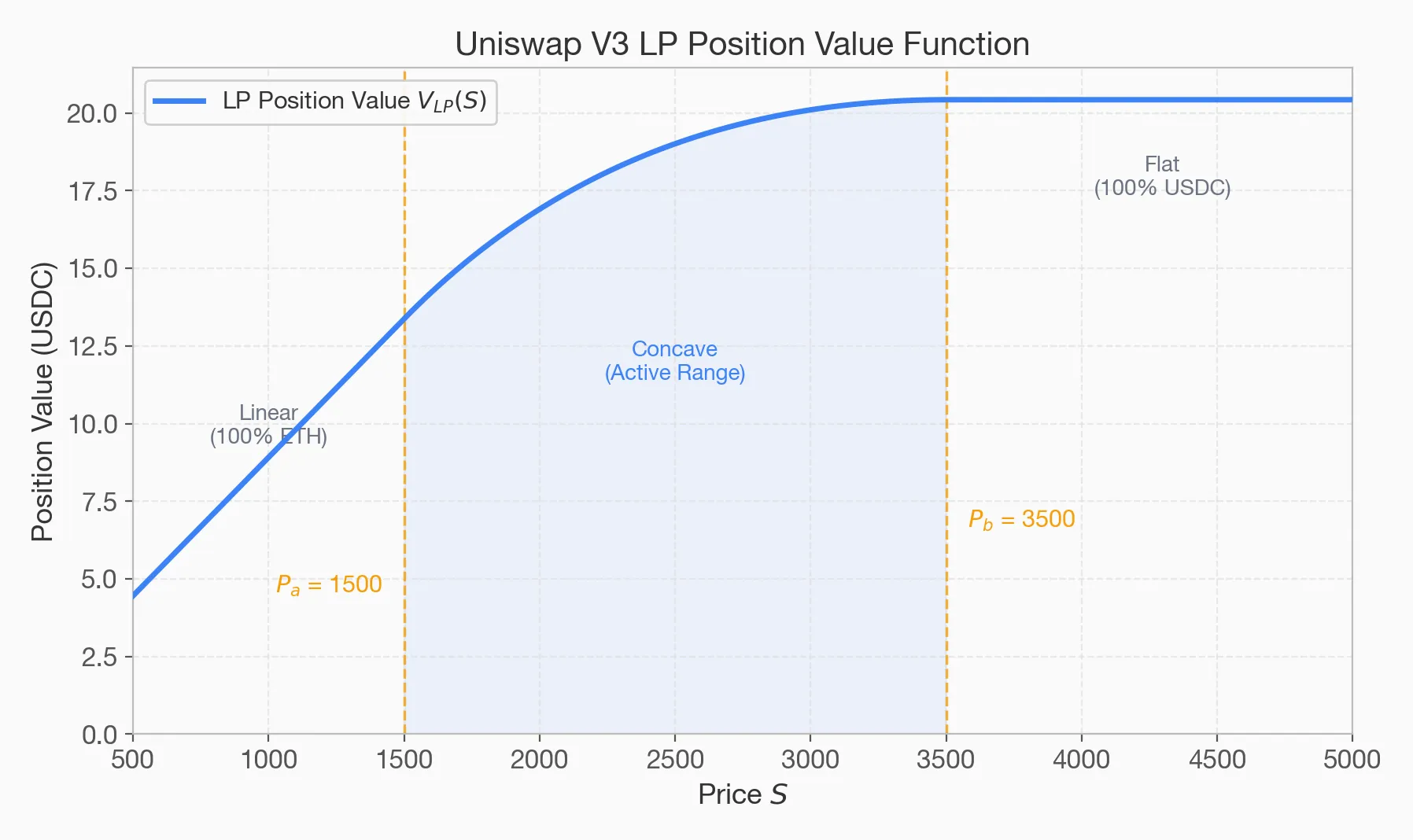
The foundation of derivatives pricing is the state equation of the underlying asset. This article focuses on Uniswap V3 as the main object of study: on the one hand, the V2 model is used less often in practice because of efficiency limitations; on the other hand, concentrated liquidity makes V3 and its variants more representative as research targets. Suppose concentrated liquidity \(L\) is provided over the Uniswap V3 interval \([P_a, P_b]\) (the V3 white paper defines \(L = \frac{\Delta y}{\Delta \sqrt{P}}\), which differs from the V2 constant-product definition \(L = \sqrt{x \cdot y}\)). The actual token holdings both inside and outside the interval are defined directly. From \(V_{LP}(S) = y(S) + S \cdot x(S)\), we can derive the piecewise total value function of the position, denominated in USDC:

$$ V_{LP}(S) = \begin{cases} S \cdot L \left( \frac{1}{\sqrt{P_a}} - \frac{1}{\sqrt{P_b}} \right) & S \le P_a \\ L \left( 2\sqrt{S} - \sqrt{P_a} - \frac{S}{\sqrt{P_b}} \right) & P_a < S < P_b \\ L \left( \sqrt{P_b} - \sqrt{P_a} \right) & S \ge P_b \end{cases} $$

Figure 1: The piecewise value function \(V_{LP}(S)\) of a V3 LP position. The \(2\sqrt{S}\) term in the middle segment determines its negative second derivative, and thus its negative-Gamma shape.

Structural Decomposition

Looking at the payoff behavior at the price boundaries, the risk profile can be understood approximately as a short strangle.

• Left boundary (\(S \le P_a\)) Once price falls below \(P_a\), the LP is forced to hold a full inventory of the depreciating asset and bears all subsequent losses. This can be understood approximately as exposure to short-put risk on the \(P_a\) side.
• Right boundary (\(S \ge P_b\)) Once price rises above \(P_b\), the asset inventory is fully converted into USDC and the LP gives up the upside beyond that point. This can be understood approximately as exposure to short-call risk on the \(P_b\) side.

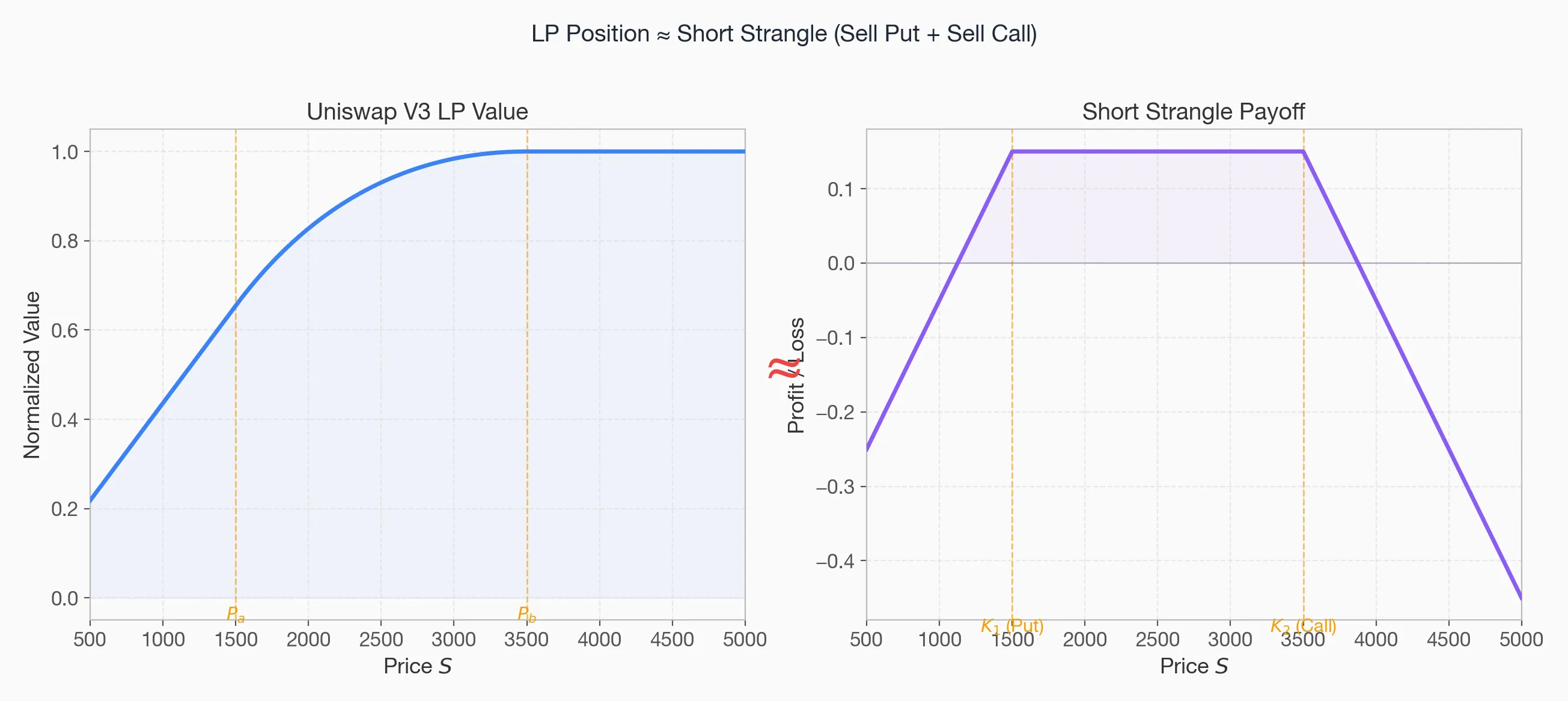
Figure 2: A schematic comparison between the V3 LP payoff (blue) and the risk profile of a short strangle (orange dashed line).

Echenim et al. show that the static essence of a V3 LP can be viewed as selling a basket of puts and calls across a range of strike prices. Its difference from a standard strangle is that, inside the interval, it also suffers continuous Gamma decay.

Valuation Models

Although the static structure is clear, the classic Black-Scholes (B-S) model cannot be applied directly to an LP position, because LP exposure has three distinctive features:

1. No fixed maturity date (perpetual nature).
2. Random stopping time (Stopping Time, \(\tau\)): the position may stop earning fees at any moment once price exits the range, so its full life cycle depends on the random time at which price first touches a boundary.
3. Embedded cash flow: continuously accrued fees during the life of the position must be discounted as an annuity.

Because the traditional “universal pricing formula” runs into these obstacles, the current literature mainly follows two complementary paths: absolute value discovery and marginal cost measurement.

Value Discovery: Martingale Stopping-Time Absolute Valuation Model (Hou et al.)

This class of models addresses the question, “What is an LP position worth right now?” It treats the LP as a singular option whose value depends on the first time the price hits a boundary.

In the derivation, the model applies a standardizing transformation to the asset price process and introduces an exponential martingale and a Laplace transform. Rather than relying purely on numerical simulation, it uses boundary conditions to derive analytical expressions associated with first-passage events.

More specifically, given the current price \(S_t\) and volatility \(\sigma\), the model first computes four intermediate parameters capturing location and decay: the drift adjustment term (\(\mu’\)), the time-decay factor (\(\lambda\)), and the standardized distances from the current price to the lower and upper boundaries (\(a’\) and \(b’\)).

Based on those variables, the present value of the LP position, \(V_t\), is finally decomposed into expected terminal asset value (the first term) and expected fee income (the second term):

$$ V_{t} = \underbrace{LP_{H} e^{\mu'b'} \frac{\sinh(a'\lambda)}{\sinh((a'+b')\lambda)} + LP_{L} e^{\mu'a'} \frac{\sinh(b'\lambda)}{\sinh((a'+b')\lambda)}}_{\text{Part 1: expected discounted principal}} + \underbrace{\frac{C_{a} L_{q}}{r} \left( 1 - \frac{e^{\mu'a'}\sinh(b'\lambda) + e^{\mu'b'}\sinh(a'\lambda)}{\sinh((a'+b')\lambda)} \right)}_{\text{Part 2: discounted fee income over the life of the position}} $$

The core of the formula lies in the probability-discount weights built from \(\sinh\), the hyperbolic sine function.

• Expected discounted principal The two terms separated by the plus sign represent, respectively, the discounted present value of “exiting at the upper boundary with all funds in USDC (\(LP_H\))” and “exiting at the lower boundary with the full position in the base asset (\(LP_L\)).” The fraction \(\frac{\sinh(\dots)}{\sinh(\dots)}\) is the Laplace-transform-based probability, with discounting, that this boundary is hit before the opposite one. For example, the closer the current price is to the upper boundary (the smaller \(b’\) becomes), the larger the probability weight of exiting with \(LP_H\).
• Discounted fee income Outside the parentheses, \(\frac{C_a L_q}{r}\) is the ideal perpetual-annuity present value under the assumption that price never leaves the interval and fees can be earned forever. But because price will eventually exit, the large expression being subtracted inside the parentheses is precisely the expected loss of fee income caused by the possibility that fee accrual may stop at any moment once a boundary is hit.

Numerical example

Take the ETH-USDC 0.3% pool as an example (let \(S_t = 2000\), \([P_a, P_b] = [1600, 2400]\), \(\sigma = 0.8, r = 0.05, \mu = 0\)):

Variable	Definition	Substitution	Example value	Meaning
\(\mu’\)	\(\frac{\mu}{\sigma} - \frac{\sigma}{2}\)	\(\frac{0}{0.8} - \frac{0.8}{2}\)	\(-0.40\)	The effective drift term of the log price. Because of the volatility drag in geometric Brownian motion, even when \(\mu=0\), the median log price still drifts downward over time due to \(-\frac{1}{2}\sigma^2\).
\(\lambda\)	\(\sqrt{\frac{2r}{\sigma^2}+1}\)	\(\sqrt{\frac{2\times 0.05}{0.64}+1}\)	\(1.08\)	The discount-intensity factor. The higher the interest rate or volatility, the larger \(\lambda\) becomes, and the stronger the discounting of stopping-time probabilities.
\(a’\)	\(\frac{1}{\sigma}\ln\frac{S_t}{P_a}\)	\(\frac{1}{0.8}\ln\frac{2000}{1600}\)	\(0.28\)	The standardized distance from the current price to the lower boundary
\(b’\)	\(\frac{1}{\sigma}\ln\frac{P_b}{S_t}\)	\(\frac{1}{0.8}\ln\frac{2400}{2000}\)	\(0.23\)	The standardized distance from the current price to the upper boundary

Cost Measurement: Continuous-Installment Option Model (Singh et al.)

Unlike Hou et al., who solve for absolute present value, the model in Singh et al. does not assign the LP a direct price. Instead, it focuses on measuring the LP’s marginal holding cost. They model the LP’s dynamic exposure as selling a continuous-installment option (CIO), a perpetual American-style installment option.

Under a CIO contract, the holder must continuously pay a funding fee (\(q\)) to keep the contract alive. This mechanism provides a good fit for the LP’s continuous process of exchanging LVR, or Gamma drag, for ongoing fee income.

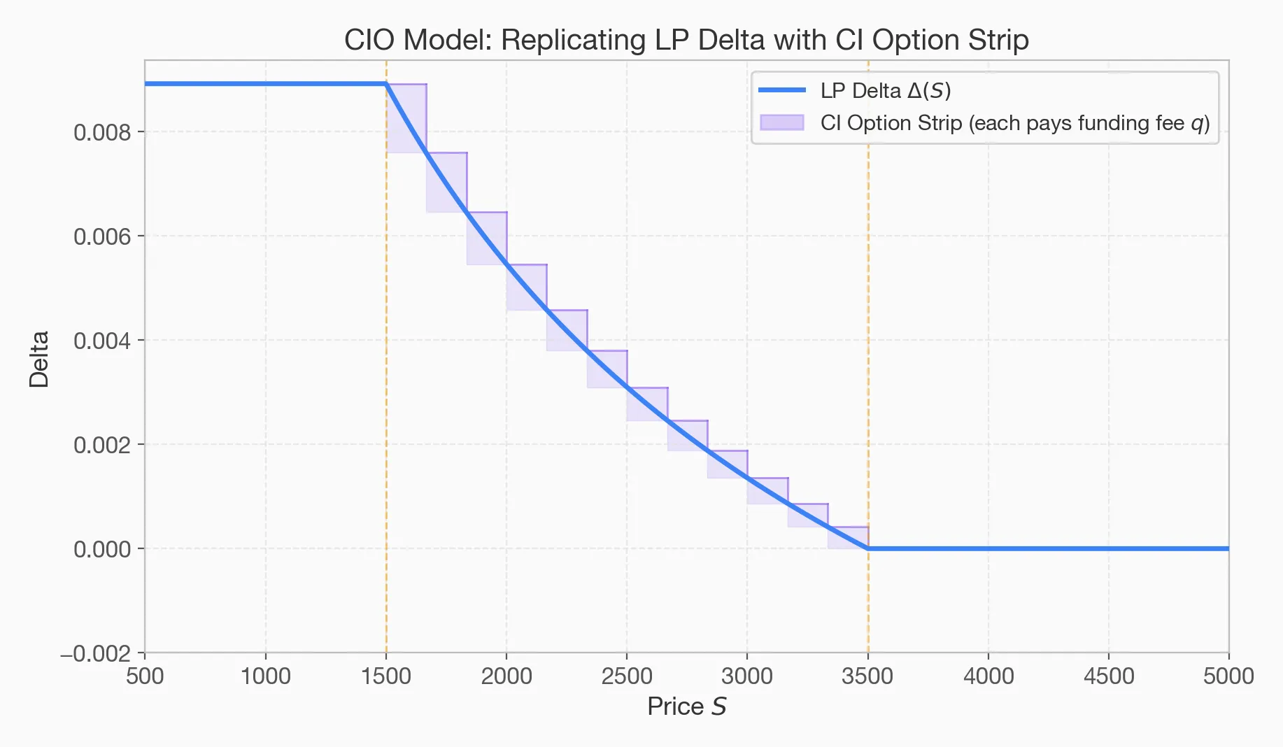
Figure 3: The LP Delta curve can be approximated by a stepped strip of CIO options.

The central identity in that paper proves that, in the limit, the total instantaneous funding-fee payments of this replication system converge exactly to the instantaneous LVR faced by the LP:

$$ d\text{LVR}_t = \text{Funding Fee} (q) = \frac{1}{2}\sigma^2 S_t^2 |\Gamma|\, dt $$

Here \(\Gamma = V’’(S_t) < 0\), so after taking the absolute value, the funding fee rate is always positive. This result provides a direct characterization of the LP’s instantaneous holding cost: fee flow is the LP’s main source of revenue, while the funding rate \(q\) can be interpreted as a theoretical expression of its core holding cost.

Greeks

Once a more rigorous framework is introduced, the Greeks can be used to describe both qualitatively and quantitatively the structural changes caused by market volatility.

Delta

Delta measures the impact of the underlying market price on the total value of the position:

$$ \Delta = \frac{\partial V_{LP}}{\partial S} $$

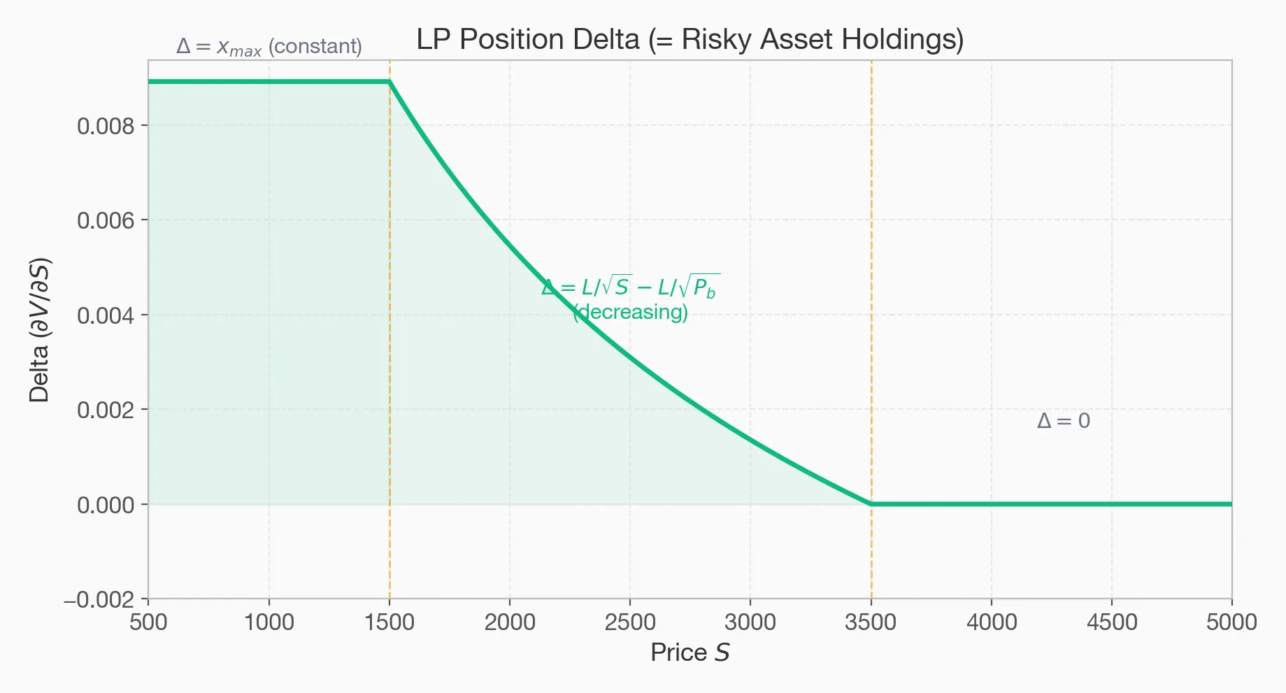
Figure 4: Delta declines with price inside the range, reflecting the automatic sell-high, buy-low rebalancing property.

But one point deserves emphasis: once the pricing formula incorporates the expected future fee income, that is, the option present-value premium, the true Delta curve diverges materially from the payoff Delta implied by the static inventory alone. Ignoring this distinction and using payoff Delta alone to guide dynamic rebalancing will often lead to under-hedging or over-hedging depending on where the current price sits inside the interval.

Gamma

Inside the interval, Gamma is always negative (\(|\Gamma| \propto S^{-3/2}\)), and this is the root cause of the continuous drawdown generated by adverse selection.

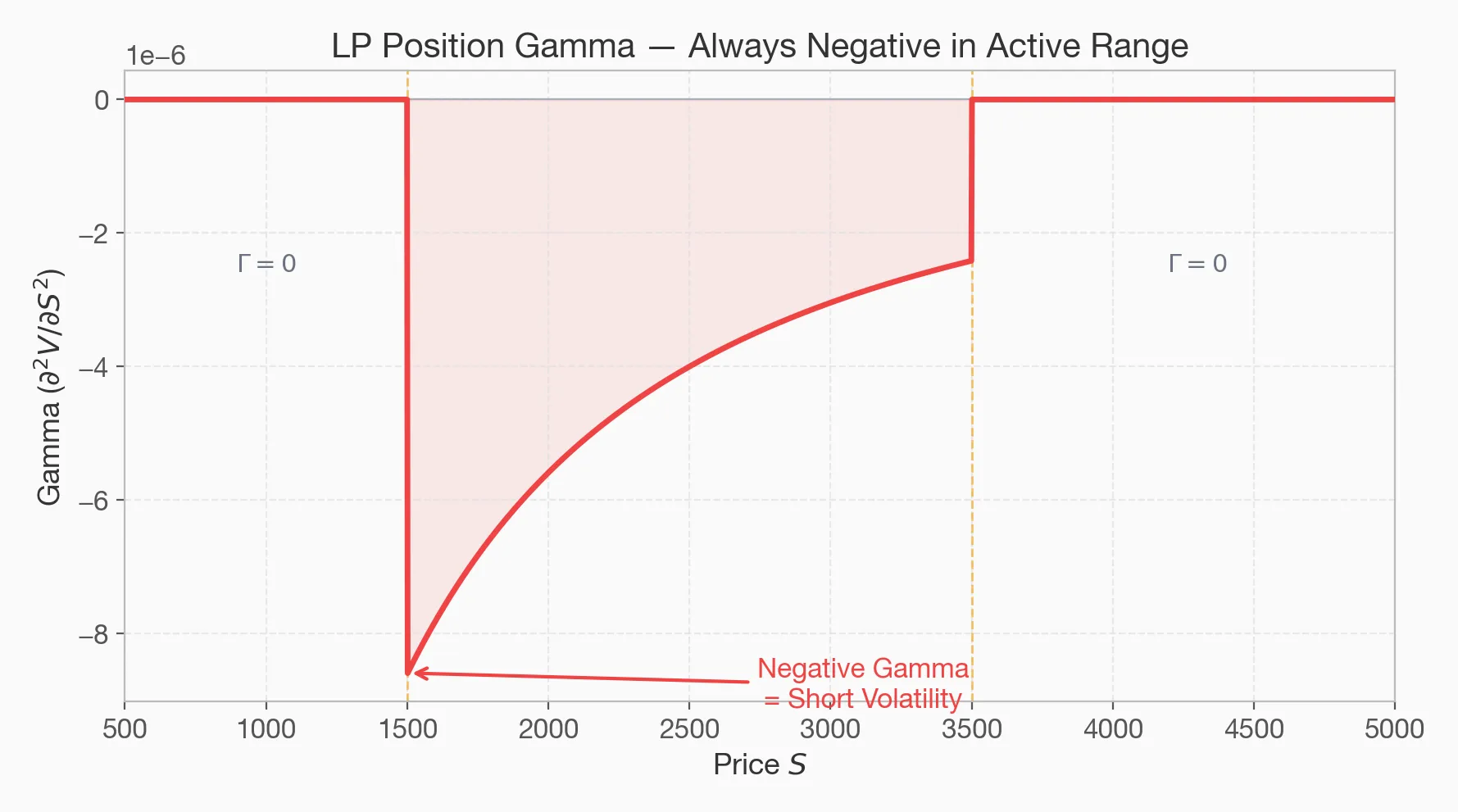
Figure 5: Gamma is always negative inside the interval, and its absolute value decays as price rises.

Substituting into the Singh identity \(dLVR_t = \frac{1}{2}\sigma^2 S_t^2 |\Gamma|, dt\) (here \(\Gamma = V’’ < 0\), exactly consistent with the notation in the previous section) confirms that the physical rate of LVR is determined entirely by price, volatility \(\sigma\), and \(|\Gamma|\). Extremely narrow ranges amplify negative-Gamma exposure dramatically, which validates the accelerated wear-and-tear caused by overly concentrated liquidity.

Vega

Being short Gamma directly implies that the LP’s Vega is also negative (\(\mathcal{V} < 0\)). Even when the current price does not move, an increase in implied volatility not only accelerates the theoretical erosion from LVR, but also immediately reduces the option present value of the position because the probability of an early boundary hit becomes larger.

Hedging and Profit

Once the position has been decomposed through the quantitative model, the LP’s final operational core is to manage Delta exposure and mitigate the loss caused by negative Gamma.

Static Hedge: Long Strangle

The original hedge proposed by Echenim is to hold call and put positions in the options market at strikes corresponding to the two price boundaries. Positive Gamma and Vega can directly offset the short-option features of the AMM. The limitation is that option funding cycles are fixed, rolling frictions can be substantial, and one must carefully assess whether current fee income is sufficient to cover option amortization.

Dynamic Hedge: Continuous Delta Neutrality

If perpetual-type instruments are used to short away directional exposure continuously, then taking the total differential of portfolio value with respect to time yields:

$$ d(\text{LP}+\text{Hedge}) = \frac{1}{2}\Gamma(S_t) \sigma^2 S_t^2 dt = -dLVR_t $$

This derivation shows that, under ideal continuous hedging, once directional risk is stripped out, what mainly remains in the portfolio is the rebalancing drag driven by negative Gamma. Dynamic hedging does not eliminate the cost; it merely makes that component of loss, which would otherwise be diffused along the price path, more explicit and more visible.

Profit Equation

Once option-overlay hedging costs are included, LP profit and loss under a given hedge setup can be written as:

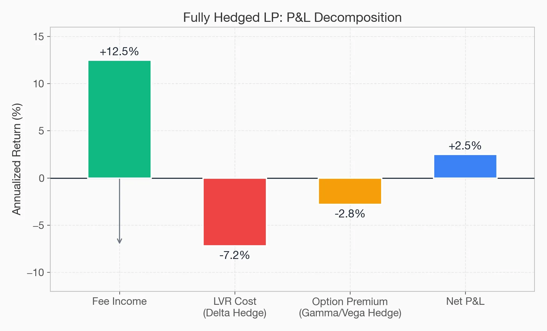
Figure 6: A three-part decomposition of LP returns under a hedging framework: fee income, LVR drag, and external hedging costs.

$$ \text{P\&L}_{\text{Hedged LP}} = \int_0^T d\text{Fees}_t - \int_0^T d\text{LVR}_t - \text{Option Premiums} $$

This option-based profit model conceptually echoes the “generalized LP fundamental P&L framework” we proposed in With the Dust of the Market: Notes on the Cultivation of a Generalized Liquidity Provider, namely \(\Pi \approx F - C_{AS} - C_{IR} - C_{Op}\), where \(F\) represents service compensation or fee income.
Within that more abstract underlying framework, the \(\text{Fees}\) earned from providing concentrated liquidity are exactly the service compensation (\(F\)); the continuously leaking \(\text{LVR}\) in the model is the adverse-selection cost (\(C_{AS}\)) paid out by the pool at the microstructural level; and the \(\text{Option Premiums}\) spent on external options to lock in the risk range constitute the structural friction and hedging cost (\(C_{IR}\)) required to eliminate inventory-drift risk.

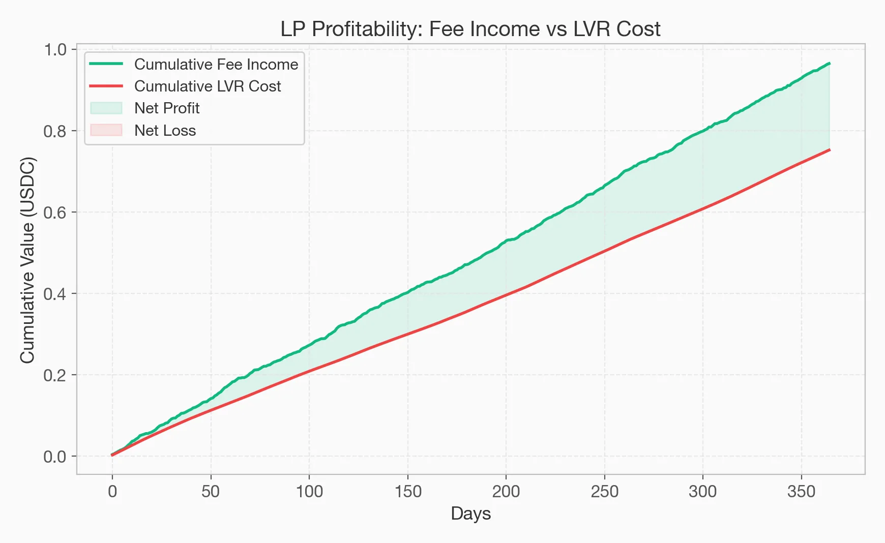
Figure 7: A cumulative P&L time series under simulated data, showing that positive net performance usually depends on relatively mild volatility and sufficiently strong trading volume.

Conclusion

Uniswap V3 LP positions have clear option-like characteristics and can be understood from several complementary perspectives: they can be related statically to option-selling structures through their payoff, and they can also be analyzed dynamically under martingale stopping-time models and continuous-installment frameworks. Under those models, fees, LVR, and external hedging costs can all be incorporated into the same accounting framework and compared directly. What rigorous hedging improves is the measurability of risk and the evaluability of strategy performance; it does not automatically imply deterministic positive returns.

Once the cards are on the table, the final sprint is optimal control at the algorithmic level. In “AMM Quant Deep Dive 03,” we will introduce the Hamilton-Jacobi-Bellman (HJB) equation from dynamic programming to derive the extremal law of the optimal interval width \(\delta_t^*\), and explore how machine learning can be layered onto the model to anticipate shifts in the underlying \(\sigma\).

---

References

• Echenim, Mnacho, Emmanuel Gobet, and Anne-Claire Maurice. n.d. Uniswap v3: Impermanent Loss Modeling and Swap Fees Asymptotic Analysis.
• Hou, Liang, Hao Yu, and Guosong Xu. 2025. “Risk-Neutral Pricing Model of Uniswap Liquidity Providing Position: A Stopping Time Approach.” arXiv:2411.12375. Preprint, arXiv, March 8. https://doi.org/10.48550/arXiv.2411.12375.
• Singh, Srisht Fateh, Reina Ke Xin Li, Samuel Gaskin, et al. 2025. “Modeling Loss-Versus-Rebalancing in Automated Market Makers via Continuous-Installment Options.” arXiv:2508.02971. Preprint, arXiv, August 5. https://doi.org/10.48550/arXiv.2508.02971.