Risk Models for Alpha Strategies: The Silent Foundation

Chinese

The role of a risk model in an alpha strategy is to predict the covariance matrix of expected returns for the underlying assets, so that portfolio variance can be minimized for a given expected return and the strategy’s Sharpe ratio can be improved. A risk model is no less important than a return model, yet compared with return modeling there is surprisingly little discussion of how to build one. One reason is that most investors simply buy commercial solutions such as Barra; another is that risk models must be judged at the portfolio level and cannot be evaluated through a simple benchmark. This article gives a systematic introduction to the definition and implementation of risk models, including shrinkage estimators, expert factor models, and data-driven statistical models.

Covariance Estimation

The Optimal Portfolio

A portfolio with high return is not necessarily a good portfolio. Modern portfolio theory tells us that the optimal portfolio is the one that delivers the highest expected return for a given level of variance. In the case of risky assets only, every feasible portfolio is a linear combination of the underlying assets, so the frontier of expected return and variance forms a hyperbola. The upper half is called the efficient frontier. Every quantitative trading strategy is, in essence, trying to move closer to that frontier and improve risk-adjusted return after combining with the risk-free asset.

Assume that the expected return vector \(\mu\) and covariance matrix \(\Sigma\) of all risky assets are known. For portfolio weights \(w\), the expected return \(R_p\) and variance \(\sigma^2_p\) are

$$ R_p = w^T \mu $$

$$ \sigma^2_p = w^T \Sigma w $$

The optimization problem is

$$ \max_w w^T \mu - \frac{\lambda}{2} w^T \Sigma w $$

where \(\lambda\) is the risk-aversion parameter. Without constraints, the optimal solution has the closed form

$$ w^* = \frac{1}{\lambda} \Sigma^{-1} \mu $$

So the problem of finding optimal portfolio weights requires estimates of both expected returns and the covariance matrix. For active management, more accurate estimation of either one can ultimately improve the Sharpe ratio and make research effort more productive.

Difficulties and Challenges

Covariance forecasting is extremely difficult in low-signal, small-sample financial data. The simplest estimate is the historical sample covariance, but the first problem is insufficient sample size. Under assumptions of normality and stationarity, estimation error causes the risk of the portfolio optimized from sample covariance to be systematically underestimated, and the relationship between estimated risk and true risk is

$$ \sigma_{\text {true }}=\frac{\sigma_{\text {est }}}{1-(N / T)} $$

As \(N\) grows, the gap becomes larger. Meanwhile, because return covariance is time-varying, it is impossible to use arbitrarily long windows of history. In stock alpha strategies, \(N\) is often an order of magnitude larger than \(T\). When the number of stocks exceeds the sample length, the sample covariance matrix becomes rank-deficient and cannot be inverted directly, which severely limits its practical value.

Even if we have a relatively reliable risk model, portfolio optimization still faces the problem of misalignment between the return model and the risk model. If the two models use different feature spaces, the return signal can be decomposed into one component projected onto the hyperplane spanned by the risk factors and another orthogonal residual component. Both affect the final optimization result, but the orthogonal component is treated as if it had no risk, which is false. That leads the optimizer to underestimate the risk of that return component. In practice, all return predictors come with correlated expected returns. In Chinese industry jargon this is often described as “profit and loss come from the same source.” Since idiosyncratic risk can be diversified away, any predictor that carries expected return but no systematic relation would imply an arbitrage opportunity, and such an opportunity would not persist for long.

Shrinkage Estimation

Can covariance estimation be made more stable by introducing structured prior information? The Ledoit-Wolf (LW) shrinkage estimator is one such method, especially useful in high-dimensional, low-sample settings. The basic idea is to combine the sample covariance matrix with a structured target matrix through a shrinkage coefficient:

$$ \hat{\Sigma}_{LW} = (1 - \alpha) \cdot S + \alpha F $$

where \(\hat{\Sigma}_{LW}\) is the shrinkage estimate, \(S\) is the sample covariance matrix, \(\alpha\) is the shrinkage intensity, and \(F\) is the shrinkage target. When \(\alpha = 0\), the method reduces to the sample covariance; when \(\alpha = 1\), it becomes the structured target. The inputs required by shrinkage estimation are simple: only historical stock return data is needed. Unlike factor models, it requires relatively little additional information.

LW defines similarity between the estimate and the true covariance using the Frobenius norm and derives the optimal shrinkage coefficient as

$$\alpha^* = \frac{\sum_{i=1}^{N} \sum_{j=1}^{N} \operatorname{Var}\left(s_{i j}\right)-\operatorname{Cov}\left(f_{i j}, s_{i j}\right)}{\sum_{i=1}^{N} \sum_{j=1}^{N} \operatorname{Var}\left(f_{i j}-s_{i j}\right)+\left(\phi_{i j}-\sigma_{i j}\right)^{2}}$$

where \(E(F_{ij})=\phi_{ij}\) and \(E(S_{ij})=\sigma_{ij}\).

Across the three classic LW papers, the authors proposed three different linear shrinkage targets \(F\).

1. Constant variance model

$$ F=I *\left(\frac{1}{T} \sum_{i=1}^{N} s_{ii}\right) $$

Using a constant-variance target is equivalent to shrinking the off-diagonal entries of \(S\) by hand.

2. Market model

The market-model target is the covariance matrix implied by CAPM, so the final estimate is a mixture of a single-factor model and the sample covariance:

$$ F=\sigma_{m}^{2} *\left(\beta \beta^{\prime}\right)+\Delta $$

3. Constant correlation model

In the constant-correlation model, the diagonal of \(F\) matches the diagonal of the sample covariance, while the off-diagonal entries are determined by a common correlation coefficient and individual stock volatilities:

$$ f_{ii}=s_{ii},f_{ij}=\overline r \sqrt {s_{ii} s_{jj}} $$

where

$$ \overline{r} = \frac{2}{N(N-1)} \Sigma_{j>i}{\frac{s_{ij}}{\sqrt {s_{ii} s_{jj}}}} $$

Expert Factor Models

One of the original motivations of multi-factor theory was to explain common movement in asset prices. Factor models assume that a sparse set of factors drives cross-sectional return differences:

$$E(R)=\alpha + \beta \lambda + \epsilon$$

So if we can estimate the factor exposures \(\beta\) and the covariance structure among factor returns, the original \(N \times N\) covariance matrix can be reduced dramatically. Let

$$ \Beta = [\beta_1 \dots \beta_N ]^T \in \mathbb{R}^{N \times K} $$

be the factor exposure matrix. Taking variances on both sides gives

$$ \Sigma = \Beta^T \Sigma_\lambda \Beta + \Delta $$

where \(\Sigma_\lambda\) is the covariance of factor returns and \(\Delta\) is the diagonal matrix of idiosyncratic volatility.

Any discussion of structured risk models for multi-factor investing eventually runs into Barra. The latter half of this section therefore focuses on stock risk models in the Barra tradition.

In the CNE5 framework there are K factors: one country factor that acts like an intercept, P one-hot industry factors, and Q style factors, so K = 1 + P + Q.

$$ R = \mathbf{1}\lambda_C + \Beta^I \lambda_I + \Beta^S \lambda_S + \Epsilon $$

One major characteristic of the Barra model is that it uses company characteristics to determine raw factor exposures, which makes computation fairly direct. For example, if a stock has returned 20% over the past year, then 0.2 becomes its raw exposure to the momentum factor. These raw exposures are then standardized by subtracting market exposure and dividing by the standard deviation, so the market portfolio has zero exposure to all factors.

Barra assumes that the variance of idiosyncratic returns is inversely proportional to the square root of market capitalization. At each cross-section it estimates factor returns \(\lambda\) using weighted least squares. Once the time series of factor returns and idiosyncratic returns is obtained, the stock covariance matrix can be computed. But a large empirical literature shows that historical estimation alone does not yield accurate covariance forecasts, so the result must be adjusted using additional statistical procedures.

Barra is widely respected in industry. As an expert-factor risk model, its main advantage is interpretability. It can be used not only for portfolio optimization but also for post hoc attribution of return and risk.

That said, structured risk models also have an inherent weakness: no human can know how many factors matter, much less enumerate all of them. The final estimate is therefore biased. This led researchers to relax the assumption that residual returns are independent, allowing \(\Delta\) to be non-diagonal. In contrast with the original exact factor model, this is called an approximate factor model.

Statistical Models

In recent years, latent-factor models based on PCA, autoencoders, and related methods have received increasing attention. If expert factor models can be understood as sparse decompositions of \(\Sigma\) based on human assumptions, then PCA is a direct data-driven decomposition of \(\Sigma\). The forms are strikingly similar. PCA decomposes the sample covariance of historical returns as

$$ \Sigma = v^T\lambda v $$

where \(v\) contains eigenvectors and \(\lambda\) contains eigenvalues. Taking the top k eigenvectors corresponding to the largest eigenvalues gives a principal-component matrix \(v^T \in N \times K\), which is structurally equivalent to the factor exposure matrix \(\Beta\).

When estimating covariance, the variance left unexplained by discarded eigenvalues is treated in PCA as idiosyncratic volatility with equal variance and added back to the diagonal of the reconstructed covariance. So PCA is, at its core, the same as the expert-factor model in the previous section, and it also shares a connection with shrinkage estimation, since LW shrinkage is equivalent to first diagonalizing the sample covariance matrix and then shrinking the eigenvalue-based diagonal matrix.

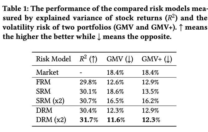
In 2021 Microsoft proposed the Deep Risk Model (DRM), which formulates latent risk-factor mining as a supervised learning problem through a specially designed loss function and achieves strong empirical results.

The paper designs a new loss to optimize three objectives in style-factor mining:

• Explanatory power The style-factor exposure matrix is learned by a neural network, \(R_{\cdot t}=g_\theta(X_{\cdot t})\), and goodness-of-fit \(R^2\) measures how much return variance is explained. So the first term maximizes empirical \(R^2\):

$$ R_{\cdot t}^{2}=1-\frac{\left\|\mathrm{y} \cdot t-\mathbf{F}_{\cdot t}\left(\mathbf{F}_{\cdot t}^{\top} \mathbf{F} \cdot t\right)^{-1} \mathbf{F}_{\cdot t}^{\top} \mathbf{y} \cdot t\right\|_{2}^{2}}{\|\mathbf{y} \cdot t\|_{2}^{2}} $$

• Orthogonality To avoid mining many nearly identical factors, the model constrains the variance inflation factor (VIF), encouraging factors to remain as orthogonal as possible. After derivation, the paper gives the equivalent form

$$ \Sigma \text{}{VIF}_i = N \cdot tr((F^TF)^{-1}) $$

• Stability The authors define the problem as a multi-objective optimization over explanatory power from 1 to 20 days ahead, which forces the learned style factors to have very high autocorrelation.

The final objective becomes

$$ \min _{\theta} \frac{1}{T} \sum_{t=1}^{T}\left[\frac{1}{H} \sum_{h=1}^{H} \frac{\left\|\mathbf{y} \cdot, \mathbf{t}+\mathbf{h}-\mathbf{F}_{\cdot t}\left(\mathbf{F}_{\cdot t}^{\top} \mathbf{F}_{\cdot t}\right)^{-1} \mathbf{F}_{\cdot t}^{\top} \mathbf{y} \cdot \mathbf{t}\right\|_{2}^{2}}{\left\|\mathbf{y}_{\cdot, \mathbf{t}+\mathbf{h}}\right\|_{2}^{2}}+\lambda \operatorname{tr}\left(\left(\mathbf{F}_{\cdot t}^{\top} \mathbf{F}_{\cdot t}\right)^{-1}\right)\right] $$

Of all the models discussed here, DRM is the one I prefer. Its definition is elegant, the input space and model structure are highly extensible, and it can make use of information such as text embeddings rather than depending only on historical return matrices. It can also take alpha predictors as input, which helps reduce the risk-return model misalignment discussed earlier.

References

• Caitong Securities, “Spark” Multi-Factor Special Report (8): covariance estimation methods for portfolio risk control and their comparison
• Ishikawa, Factor Investing
• Lin, Hengxu, Dong Zhou, Weiqing Liu, and Jiang Bian. 2021. Deep Risk Model: A Deep Learning Solution for Mining Latent Risk Factors to Improve Covariance Matrix Estimation. arXiv. http://arxiv.org/abs/2107.05201.