Quant 4.0 (III): Explainable AI, Knowledge-Driven AI, and Quantitative Research

Chinese

XAI (Explainable Artificial Intelligence) has been an important research direction for decades and is crucial to the credibility and robustness of artificial intelligence models. In the quantitative field, improving the explainability of AI can make decision-making processes more transparent and easier to analyze, provide researchers and investors with useful insights, and uncover potential risk exposures. In this article, we will discuss how to leverage XAI in Quant 4.0: the first part introduces common XAI techniques, and the second part connects these techniques to practical quantification scenarios. Knowledge-driven artificial intelligence is an important complementary technology to data-driven artificial intelligence, especially in low-frequency investment scenarios such as value investing and global macro investing. At the end of this article, we introduce how to apply knowledge-driven artificial intelligence to quantitative research.

This article is a partial translation of the paper Quant 4.0: Engineering Quantitative Investment with Automated, Explainable and Knowledge-driven Artificial Intelligence, with some deletions. Original address

Quant4.0 (1) Introduction to quantitative investment, from 1.0 to 4.0

Quant4.0 (2) Automated AI and Quantitative Investment Research

Quant4.0 (3) Explainable AI, knowledge-driven AI and quantitative investment research

Quant4.0 (4) System integration and simplified version of quantitative multi-factor system design

Learn about explainable AI

XAI is an emerging interdisciplinary research field covering machine learning, deep learning, reinforcement learning, statistics, game theory and visualization. Here, we focus on two types of XAI: model-intrinsic interpretation [128] and model-agnostic interpretation [129].

Model intrinsic explanation in XAI

Risk control and risk management are important tasks in the financial industry. When AI models are deployed in real-world applications, regulators often require transparency into their decision-making processes to ensure the safety of transactions. Additionally, many large financial institutions, such as banks and insurance companies, require models to be inherently interpretable.

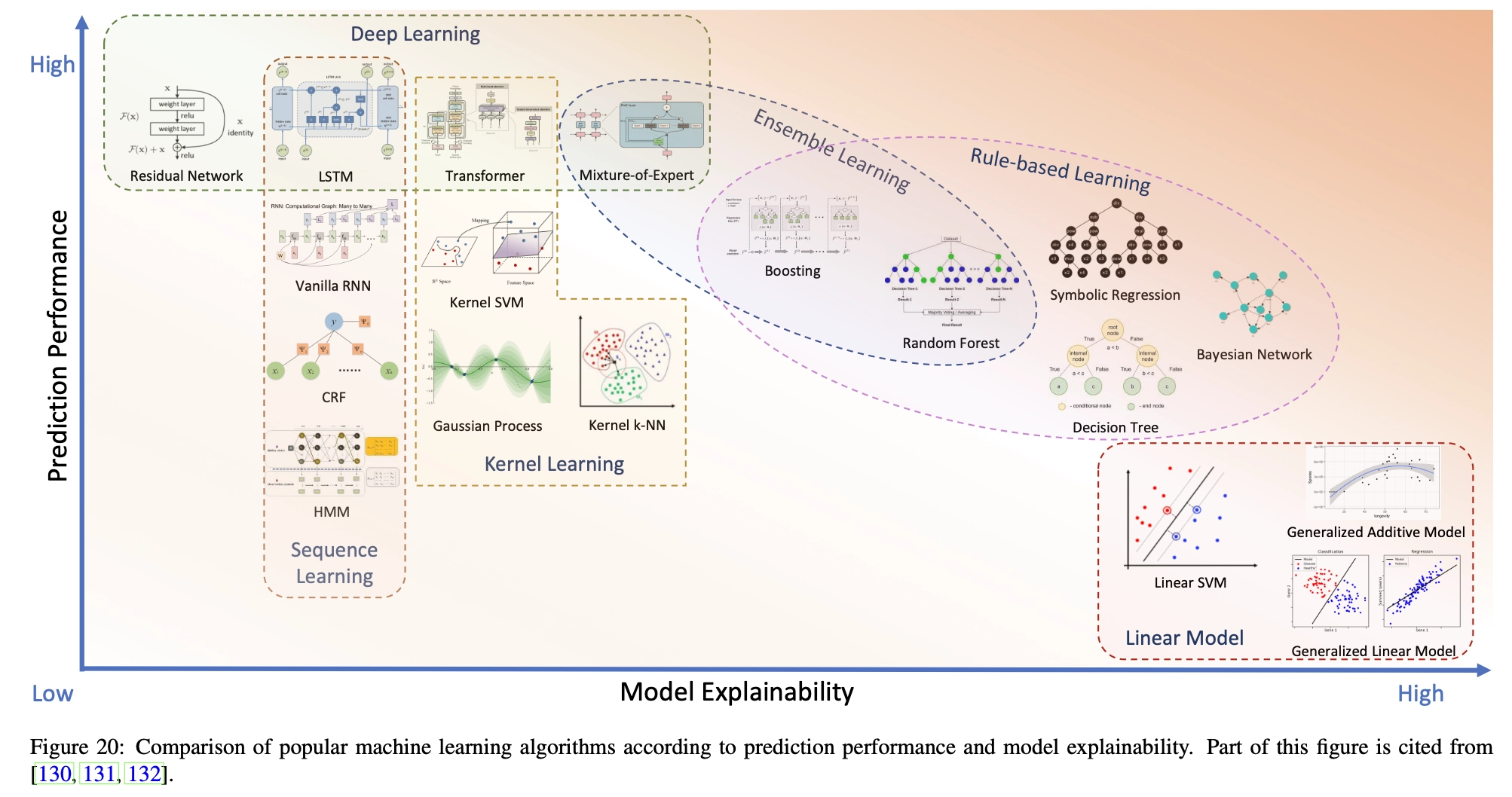
A machine learning model is inherently interpretable if its internal structure or mechanism can be easily explained. Some machine learning algorithms, such as linear models and decision trees, are inherently interpretable, while others, such as deep neural networks and kernel learning methods (SVM, Gaussian processes, etc.), are black boxes with poor interpretability. Figure 20 shows a number of popular machine learning methods, ranked according to their general performance and interpretability. We can see that improving the intrinsic interpretability of the model usually leads to a decrease in the model’s predictive performance, so choosing a machine learning algorithm is essentially a trade-off between interpretability and performance. We briefly introduce some typical machine learning methods and discuss their applicable scenarios from the perspectives of interpretability and predictive performance.

• Linear models, such as linear regression, logistic regression, linear discriminant analysis, linear SVM and additive models, are a class of methods in which the transformation of features or feature groups exists in additive form, so that the performance of the final prediction can be easily attributed to the influence of individual features or feature groups. Therefore, linear models are inherently understandable and interpretable. For example, linear regression explicitly encodes the importance of each feature, which corresponds to its regression coefficient (assuming each feature is normalized to eliminate scale and unit effects). Although linear models are easy to interpret, they perform poorly in predictive performance because they cannot encode complex nonlinear relationships between predictive outputs and features.
• Rule-based learning is another type of approach that is easy to explain. Unlike linear models that fit linear decision boundaries, rule-based learning methods fit piecewise decision boundaries composed of decision rules that combine many logical expressions. Rule-based learning includes decision trees [133], symbolic regression, and ensemble models such as random forests [134] and Boosting [135, 136, 137]. Rule-based learning models are inherently interpretable decision rules that are close to the logic of human thinking processes. However, to better fit the training data and improve prediction performance, decision rules are often more complex, which reduces interpretability and increases the risk of overfitting.
• Ensemble Learning combines multiple machine learning algorithms to achieve better decision-making performance than a single model. Typical examples of ensemble learning include random forests and boosted trees, which combine multiple tree models and make predictions based on the aggregation of individual decisions. Despite the controversy, in this paper, we also classify Mixed Experts (MoE) as an ensemble learning model. MoE combines multiple expert networks in parallel at one level and determines which expert (or experts) participates in the decision-making of a specific data point through a gating mechanism. Compared to other machine learning methods, ensemble learning provides a high level of interpretability by showing the relative importance of individual models or experts.
• Kernel Learning, also known as kernel method or kernel machine, is a type of non-parametric learning method that makes predictions by calculating similarities between samples. The similarity is described by the kernel function, which is a special inner product defined in the high-dimensional Hilbert space into which the original data samples are mapped [139]. For example, kernel support vector machine (SVM) [140] transforms the original positive/negative samples into another space so that they can be easily separated by linear decision boundaries. In principle, the kernel function can be of any form that satisfies Mercer’s conditions [141], which determine the nonlinear relationship between input and output. Furthermore, the concept of kernel function is extended to neural networks, such as the self-attention mechanism used in Transformer [142]. Traditionally, we believe that kernel tricks improve model performance but weaken its interpretability. However, from another perspective, the definition of the core itself encodes the user’s prior insights and helps in understanding the model.
• Sequence Learning refers to a class of machine learning methods that work with sequential data, such as time series or sentences. They are widely used in areas such as speech recognition, language understanding, DNA sequence analysis, and stock price prediction. Sequence learning methods characterize the hidden structure in sequence data and discover implicit patterns. For example, Hidden Markov Models (HMM) [144] assume that the underlying structure is a homogeneous Markov chain determined by a transition matrix (or transition kernel of a continuous state space), and assume that the observed sequences are randomly generated from this chain through emission probabilities. During model training, the transition probability matrix and emission probability are estimated. Although an HMM is typically a black-box model, its transition probability matrix provides some insights into the autoregressive structure in predictions. Conditional Random Fields (CRF) [145] extend the first-order Markov assumption of HMM and use a graphical model of probabilistic modeling to characterize longer range time dependencies. This additional flexibility usually leads to better prediction performance for CRF. Recurrent neural networks (RNN) such as LSTM [146] and GRU [147] perform better in sequence prediction, but explaining their internal mechanisms is more difficult.
• Deep learning often has excellent predictive performance [148], but its lack of interpretability is obvious. Some special operators in deep neural networks, such as convolution and attention, provide partial and local explanations about their mechanisms. For example, the self-attention layer in Transformer [143] characterizes the relative importance of each position in the sequence relative to other positions.

The inherent interpretability of machine learning models is always at odds with its predictive power. However, until new machine learning models emerge with both high predictive accuracy and high interpretability, we can reconstruct and improve current machine learning methods. We can start with an interpretable model (such as a linear or rule-based model) and improve its predictive performance by introducing more local nonlinear structures with better predictive power. For example, starting from a decision tree model, we can replace the decision rules in each leaf node with a neural network [149], thus increasing the flexibility of the model. As another example, starting from a deep neural network, we can also improve its partial interpretability by introducing a special layer (such as a self-attention layer [150]) to identify which important features interact more frequently.

Model-independent interpretation in XAI

To resolve the tension between performance and interpretability, a suboptimal solution is to relax the requirements and move from model-intrinsic to model-independent explanations. According to the scope of interpretation, model-independent XAI can be divided into global methods (explanation is applied to all samples) [151] and local methods (explanation is applied to some samples) [154].

Global methods explain the properties of features relevant to all samples in the dataset. These properties include feature importance, feature set importance, feature interaction effects, and other higher-order effects of features. There are various types of methods for estimating global feature importance.

• Feature Marginalization Method estimates the importance of a specific feature or a specific set of features by marginalizing all other features in the model. Specifically, the importance of the first feature is calculated by integrating over all other features, similarly we calculate the second feature, the third feature, etc. For example, Partial Dependence Graph (PDP) [135] computes the marginalized model function based on the features of interest and visualizes the corresponding feature importance. Accumulated local effects (ALE) plots [155] provide unbiased estimates of marginal effects using conditional distributions that take into account correlations between features.

• Feature Leave One Out evaluates the importance of features of interest by comparing the difference in model performance before and after removing those features from the data. Specifically, features of a model can be removed by shuffling their values ​​across samples [134, 156]. The leave-one-out approach can also be extended to evaluate interaction effects of features. For example, based on the partial dependence function, the H statistic [157] was proposed to test the interaction between features. Other alternative techniques for evaluating and visualizing feature interactions have also been proposed in [158, 159]. Additionally, we can perform functional decomposition [158] on the original model to explore interactions between all possible feature sets.

• Feature surrogate methods explain the model by learning a globally interpretable surrogate model [160] that approximates the original model. The surrogate model is trained using the dataset under the supervision of the original model, where the inputs are kept constant and the outputs are generated by the original model.

Figure 21 summarizes popular global interpretation methods, some of which have been introduced above. Furthermore, these approaches can be classified as data-driven and model-driven, with the former treating the model as a black box and querying the model to obtain explanations, while the latter treating the model as a white box and using internal information (such as gradients) to provide explanations.

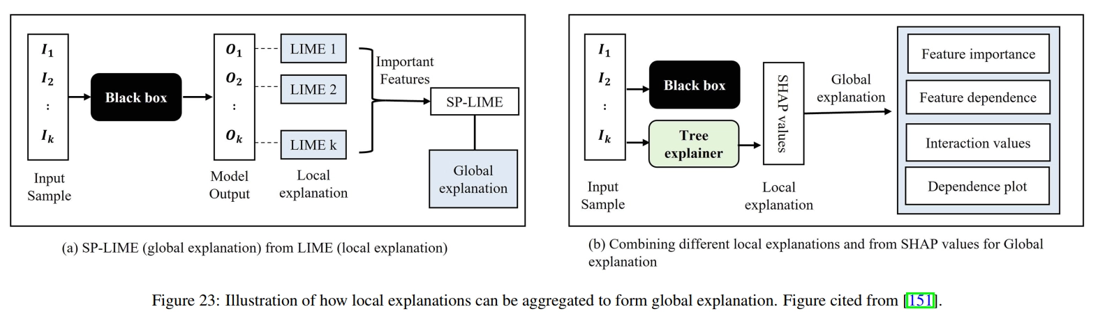
Local methods explain feature importance at the sample level, that is, how important a feature of a specific sample is to it. Similar to local dependence graphs, we can plot individual conditional expectation (ICE) graphs [161] for each sample, which illustrate the impact of the feature of interest while fixing the values ​​of other features at specific values. To explain a black box machine learning model at a specific sample, we can learn an alternative model near the data sample to locally explain the original model. Typical examples include LIME [152] and Anchors [153]. In LIME (Fig. 22), LASSO regression [162] is used as a surrogate model to fit random samples generated by perturbing the original samples around specified samples. In this way, the samples selected by this local LASSO model contribute the most to the fitness of the specified sample. Similar to LIME, anchors are interpretations of individual samples given in the form of IF-THEN rules [153] involving features. These anchors are generated by iteratively adding features to the rules using beam search. In each iteration, the candidate with the highest estimated accuracy is retained and used as the seed for the next iteration. Additionally, we can use feature importance to provide local explanations. For example, SHAP [163] proposes a unified framework for calculating the importance of each feature in a sample using Shapley values ​​[164]. Due to the high computational cost of accurately calculating SHAP values, SHAP also proposes several approximate methods to accelerate estimation. Gradient information can also be applied to differentiable models, such as deep neural networks, to illustrate the importance of input features to model predictions. As shown in Figure 23, local interpretations such as LIME and SHAP can also be aggregated into global interpretations. Such global explanations can form dataset-level explanations by aggregating explanations across all samples. For example, by calculating the average importance of each feature across the entire dataset, we can identify important features that contribute significantly to model predictions for the majority of samples in the dataset.

Explainable AI in Quant

Stock explanation

Explanations can be provided for given stocks to illustrate their sensitivity to different factors at different times and the relationships between them. Some tasks regarding stock interpretation are as follows:

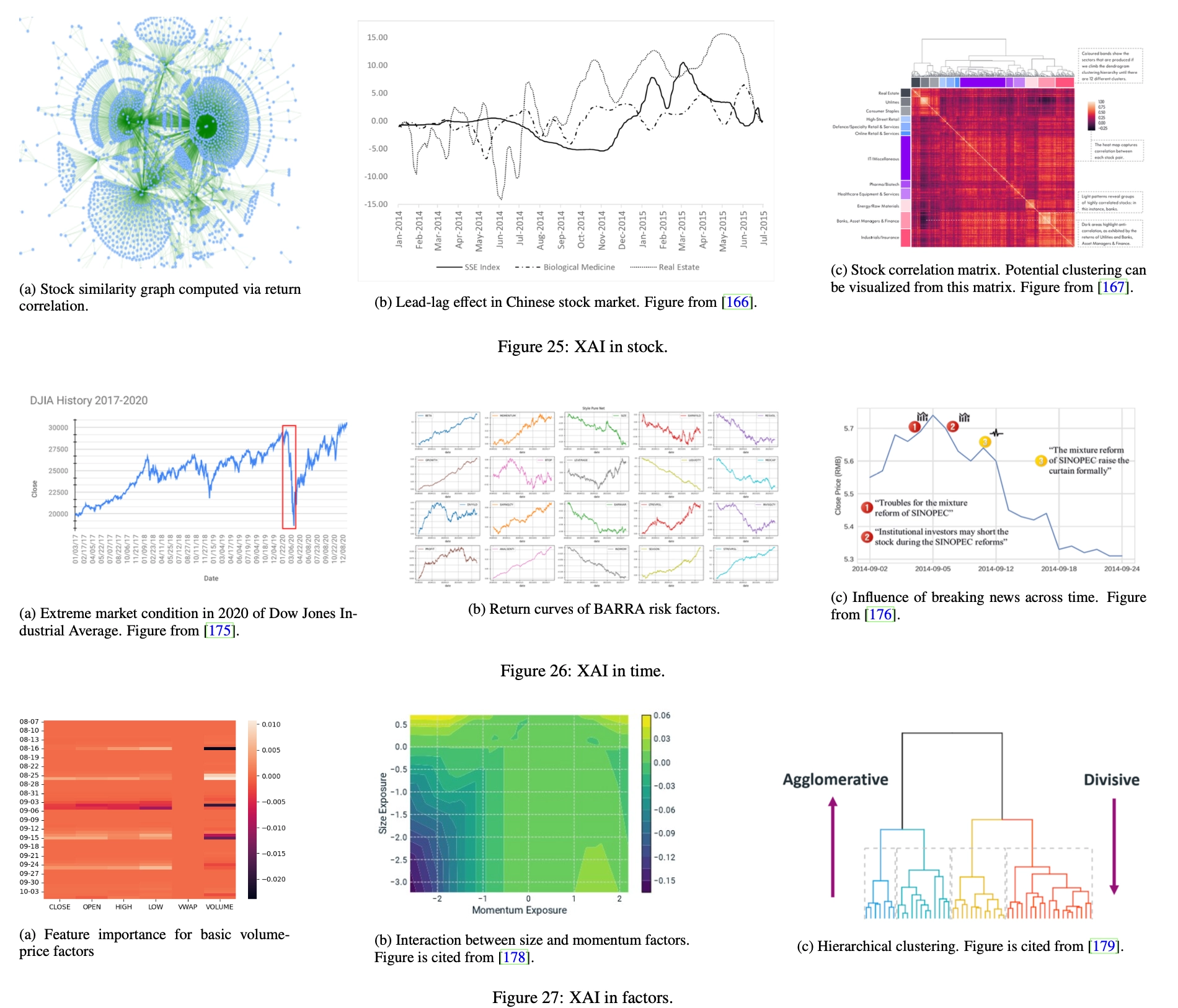
Stock Similarity Stocks are generally related in many ways (as shown in Figure 25a), and related stocks are expected to share common characteristics. In this sense, exploiting relationships between financial instruments can provide analytical and predictive advantages over the traditional approach of treating stocks individually. By analyzing the similarities between stock embeddings, we can also better understand what the model has learned. However, the challenge lies in identifying a suitable similarity measure, which needs to be sufficiently flexible and efficient. This problem is related to metric learning [168, 169] and graph structure learning [170]. A good similarity measure between stock embeddings is needed. Based on this metric, the graph structure can be constructed by computing an adjusted adjacency matrix based on pairwise similarity.

1. Stock similarity can be used to predict the covariance matrix
2. Similar momentum effects among stocks are a source of alpha

Leader-lag effect In the lead-lag effect [171], the trend of a certain stock is followed by some other stocks with a lag in time. When following the lead-lag effect, investors can observe trends (i.e. price increases/decreases) in leading stocks and take corresponding positions on lagging stocks before the same trend replicates. In this way, investors can profit by accurately identifying lead-lag effects in the market [172, 173]. However, identifying lead-lag effects is not a trivial task because copying trends often occur in financial markets, but only a few of them are actually caused by lead-lag effects. Rigorous identification of lead-lag effects requires causal inference, which requires counterfactual interpretation [174]: What would have been the trend in lagging stocks if the leading stocks had not behaved this way? However, in real-world financial markets, counterfactual reasoning is often not feasible.

Capture investor underreaction

Sector Trends Sectors are classifications of stocks defined based on certain criteria, such as industry and market capitalization. Stocks in the same sector share certain common characteristics, and the trends of individual stocks may be affected by the sector to which they belong. Therefore, it is crucial to identify the contribution of sectors to individual stocks. To do this, we can treat a stock’s affiliation to different sectors as categorical features and calculate the importance of these factors through a feature importance algorithm. In addition, investors can understand the characteristic interactions between sector affiliation and other common characteristics by assessing the sensitivity of sectors to different types of characteristics.

Time explanation

Explanations can be calculated at individual points in time to account for stocks and factors at that cross-section, and explanations across cross-sections can be further combined to provide insights into market style over a period.

Extreme Markets In the stock market, extreme conditions exist where almost all stocks in the market experience severe price declines (as shown in Figure 26a). In extreme markets, it is difficult for quantitative strategies to achieve excess returns because the prices of all stocks fall at the same time, leaving little room for arbitrage. Therefore, in extreme markets, it is crucial to identify less affected stocks and trade them for outsized returns. To accomplish this, we can break down stock returns in two ways: the contribution of market trends and the contribution of stock-specific characteristics. The decomposition can be calculated by dividing the factors into market factors and stock-specific factors. The importance of these two factors can then be calculated through the feature importance algorithm. We need to select those stocks where the importance of stock-specific factors outweighs the importance of market factors.

It can be achieved using PCA to correlate Stock Idiosyncratic Risk

Calendar Effect The calendar effect [177] refers to market anomalies related to calendars, such as days of the week, months of the year, and periods related to events, such as the U.S. presidential cycle. The calendar effect is caused by market participants’ expectations of future trends and has a great impact on market trends. Therefore, it is important to identify calendar effects in quantification and use them to adjust investment strategies. This type of identification can be achieved through the feature importance algorithm. By calculating the importance of calendar factors, such as categorical features representing weekdays and days of the month, we can see whether model predictions depend heavily on these features. Greater importance for calendar factors generally indicates potential calendar effects.

A shares also have obvious calendar effects

Style Shift Style factors are used in multi-factor models (as introduced in §1.4) such as BARRA [48] to describe the intrinsic characteristics of stocks, such as size, volatility, growth, etc. In this model, a stock’s return is contributed by its exposure to these style factors, and the return contribution per unit of exposure, also known as factor return, differs among style factors. In addition, the returns of each factor will also change over time (Figure 26b), as the market’s preference for different styles changes. If this shift can be accurately identified, investors can adjust their strategies accordingly, focusing on stocks with greater exposure to dominant style factors. To detect style shifts, we can treat style exposure as a factor and calculate its contribution to stock returns using a feature importance algorithm. We can then observe the distribution of factor contributions over time and detect changes in this distribution as signals of style shifts.

Factor timing is difficult, but also fascinating

Event Impact Unexpected events (Figure 26c) usually have a significant impact on the stock market. Investors need to deeply understand the impact of unexpected events in order to reduce the negative impact or profit from it. Typically, an event is associated with two pieces of information: the timestamp of its occurrence and specific content, which is often represented in natural language. Event content can be encoded into specific factors using natural language processing techniques [176], and the impact of an event can be calculated as the importance of content factors related to market trends after its timestamp. Additionally, we can calculate causal explanations to show the causal effects of events.

Factor explanation

Each factor can be interpreted to illustrate how different stocks are sensitive to it at different times. Explanations can be combined to show the interactive effects between specific stock factors.

Factor Types Factors can be classified in various aspects. For example, from the perspective of data sources, factors can be classified into volume-price factors, sentiment factors, basic factors, etc. From the perspective of financial characteristics, factors can be classified into momentum factors, mean reversion factors, lead-lag factors, etc. From the perspective of time scale, factors can be classified into scale-level factors, minute-level factors, daily-level factors, etc. The contribution of different types of factors to portfolio returns can be calculated through feature importance algorithms, providing investors with a better understanding of AI-generated investment strategies. For example, in Figure 27a, the contribution of each factor to the model predictions in different time windows is presented as a heat map.

Factor interaction Deep learning models are good at capturing the complex associations between factors, and some weak factors can be combined to form strong factors. This interaction reflects interesting patterns among factors and provides new insights into finding new factors. Feature crossover techniques can be used to reveal interactions between factors. For example, in Figure 27b, a landscape map of model predictions with respect to two factor values ​​(Exposure to Scale and Momentum Style factors) is presented as a contour plot. As can be seen from the map, as the values ​​of both factors decrease, the model predictions also decrease.

Factor Hierarchy We can depict the semantic similarity between factors in a hierarchical manner. Utilizing related techniques, such as hierarchical clustering [180], factor evolution graphs demonstrate the relationships between factors by arranging factors with higher similarity in lower-order neighborhoods (lower-level subtrees in the example in Figure 27c).

Knowledge-driven AI in Quant

In this part, we will introduce and demonstrate the application of knowledge-driven artificial intelligence in Quantification 4.0 from two aspects: the construction of financial behavior knowledge graphs and quantitative knowledge graph reasoning.

Build a financial knowledge graph

Ontology Design The ontology of the financial behavior knowledge graph should cover the following aspects of information:

1. Basic information of financial entities
2. Financial events occurring between financial entities
3. Causal relationships between entities and events

Entity categories include but are not limited to:

• Financial entities, including stocks, bonds, banks, listed companies, important individuals, commodities, etc.
• Concepts that reflect basic information about financial entities, such as sectors, industries, exchanges, regions and countries, currencies, etc.
• Events, that is, economic actions, such as administrative penalties, illegal acts, litigation status, changes in shareholdings, personnel changes, etc.

Likewise, categories of relationships include, but are not limited to:

• Relationships between entities, such as subsidiaries, affiliations, shareholdings, etc. These relationships are associated with timestamps, indicating when they start and end. For example, in Figure 28, the industry chain and capital chain relationships describe the department classification and capital relationships between entities.
• The relationship between events, such as co-occurrence and sequential occurrence.
• The relationship between events and entities. For example, in Figure 28, negative coverage resulted in price changes, further investigation into “Pharmaceutical Company A,” resulting in trading suspensions and litigation. Causal relationships are often inferred from existing knowledge as important auxiliary information in downstream reasoning tasks. For example, in Figure 28, the “related” relationship connects the “negative coverage” event and the corresponding financial entity “Pharmaceutical Company A”, indicating that a negative report occurred to the listed company “Pharmaceutical Company A”. These relationships are often associated with timestamps, indicating the specific point in time when an event occurred.

Knowledge Acquisition The knowledge that constitutes the financial behavior knowledge graph can be obtained from various sources, and the most challenging part is to extract useful structured knowledge from unstructured data (represented by text data). Natural language expressions are highly flexible and personalized, so it is a challenge for machines to accurately understand the information in documents and extract the most useful knowledge to build knowledge graphs. There is a large amount of contradictory information in news and documents, making fact extraction difficult. Therefore, probabilistic models and machine learning models play an important role in knowledge extraction with confidence evaluation. Furthermore, the information is often incomplete, requiring inferences about the knowledge we are actually interested in. Therefore, missing knowledge also needs to be inferred from the given facts. Different data sources often have inconsistent update frequencies, which brings new challenges to the appropriate representation of knowledge graphs. Both snapshot-based representations and log-based flat knowledge graphs can capture temporal information. Log-type floor plans are friendly to time updates, but it is difficult to directly perform time analysis on them. In contrast, snapshot-based representations are naturally suitable for temporal analysis, but also bring additional costs in terms of storage and management.

Quantitative knowledge reasoning

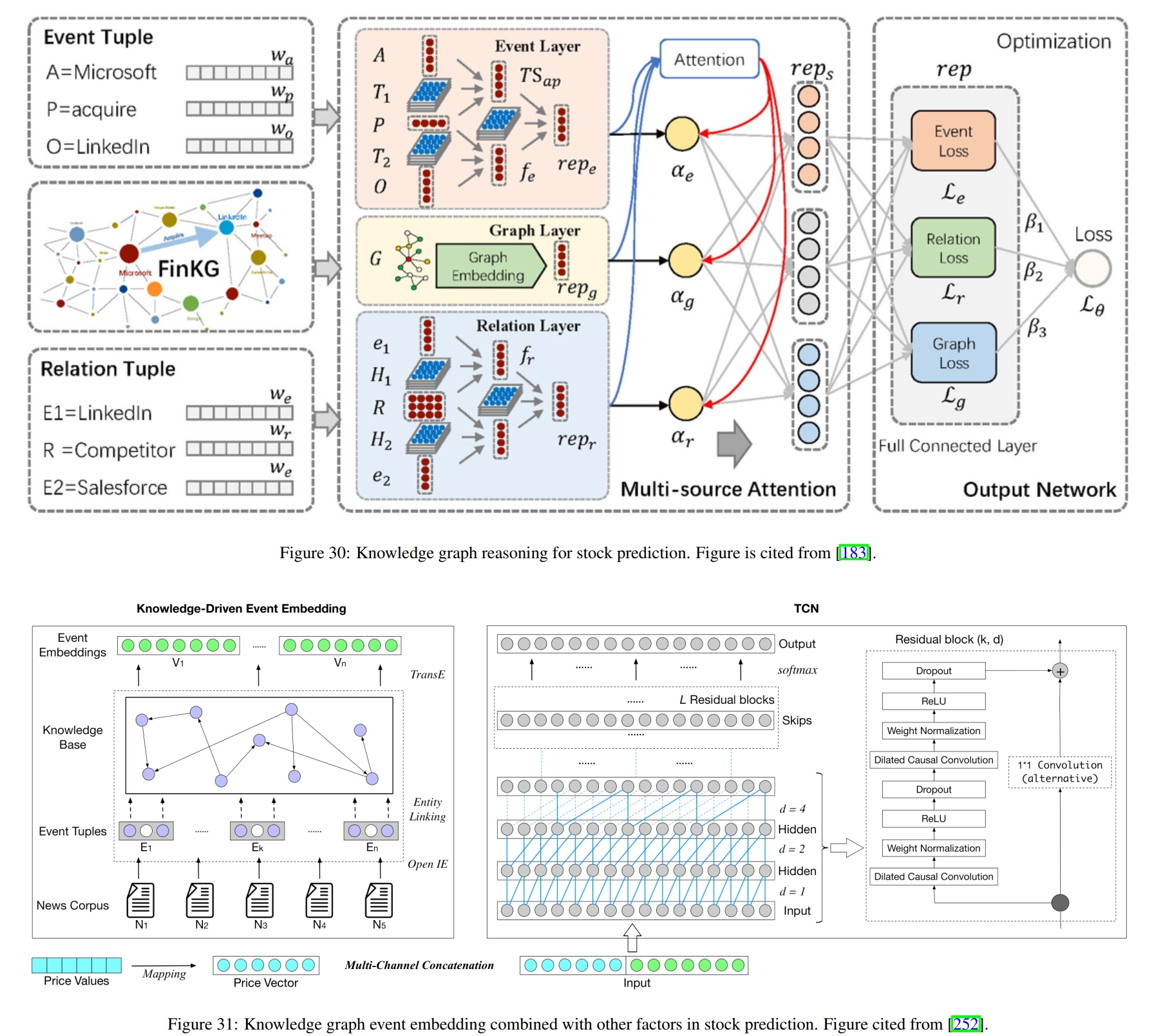
Given a knowledge graph, we can obtain meaningful knowledge representation by reasoning on the graph. For quantification, knowledge representation can be incorporated into existing factors as external information and fed to deep learning models for better predictions. Figure 30 shows the typical process of knowledge reasoning in quantification. Specifically, events and relationships between stocks are represented as semantic triples, where entities and relationships are embedded into vectors. Then, neural inference is performed on these semantic triples to compute embeddings of events, relationships, and the entire knowledge graph. After training on historical data, the knowledge representation is used in investment strategies to generate trading decisions.

There are other studies devoted to the application of knowledge reasoning to quantification. [253] proposed to incorporate relational and categorical knowledge into event embeddings to obtain better results. Given a semantic triple representing an event, external information about the entities in the semantic triple is retrieved from the knowledge graph and incorporated into the computation of the event embedding. [252] extract events from news text and align the extracted information with the knowledge graph using entity linking technique [254]. Then, use TransE to generate event embeddings. The embedding is then combined with volume-price data in a temporal convolutional network [255] for stock prediction, as shown in Figure 31. [53] utilize basic information such as sector classification and supply chain to construct a knowledge graph and calculate the embedding of each stock using temporal graph convolution. These embeddings are then used to predict stock returns and the entire model is trained by maximizing the stock ranking loss. [256] use node2vec [257] to generate stock embeddings based on knowledge graphs and use these embeddings to calculate similarities between stocks. In this way, the top K nearest neighbors are calculated for each stock, and the neighbors’ factors are used to augment the original factors. Other studies [258, 259] also leverage knowledge graphs to generate better stock embeddings or make event-driven investments.