Quant 4.0 (II): Automated AI and Quantitative Research

Chinese

The automated AI in Quantification 4.0 covers the automation of the entire quantitative process. In this section, we first introduce the overall view of the R&D process, and then discuss how to upgrade it to an automated AI version.

This article is a partial translation of the paper Quant 4.0: Engineering Quantitative Investment with Automated, Explainable and Knowledge-driven Artificial Intelligence, with some deletions. Original address

Quant4.0 (1) Introduction to quantitative investment, from 1.0 to 4.0

Quant4.0 (2) Automated AI and Quantitative Investment Research

Quant4.0 (3) Explainable AI, knowledge-driven AI and quantitative investment research

Quant4.0 (4) System integration and simplified version of quantitative multi-factor system design

Automated investment research process

Traditional process

Decades of development have resulted in a standard workflow for quantitative research, as shown in Figure 11 (blue part). This workflow includes many modules, including data preprocessing, factor mining, modeling, portfolio optimization, order execution, and risk analysis.

Data preprocessing is usually the first step in quantitative research. There can be many problems with the raw data. First, financial data often have some missing records. For example, in technical analysis, you may not receive price data at certain points in time due to packet loss during communication, or miss price data on certain trading days due to a stock suspension. Likewise, in fundamental analysis, you may miss portions of financial statement data because it is not reported in a timely manner. Although traditional statistical data imputation methods can be used to impute and fill in missing records, the use of future information must be avoided during the imputation process. Second, financial data contains extreme values ​​and outliers that may come from erroneous records, data storage issues, data transmission issues, or extreme markets, and these outliers can lead to risk biases in investment decisions. Outliers can be eliminated by the data winsorization method [43], which limits extreme values ​​within a certain percentile range, but it must be noted that some outliers are actually strong signals of quantitative trading rather than noise, and the two must be distinguished during data preprocessing. Third, many financial data, such as news event data, have low data coverage and irregular update frequency. We must align these types of data with high coverage and regular frequency data (such as market data) to facilitate downstream factor mining and modeling tasks. Fourth, different data features vary greatly in value range, so some “big” features may dominate in modeling. Therefore, data normalization methods are used to normalize the range of features. Care must be taken in the way data are normalized to reduce information loss.

The article is mainly written for deep learning models. In fact, the gradient boosting tree model does not require these data preprocessing.

Factor mining is a task of feature engineering [44] that leverages knowledge from the financial and economic fields to design, search, or extract factors (features for downstream modeling) from raw data. Generally, larger factor values ​​indicate more significant trading signals. The motivation for factor mining is to find these signals from raw data for market prediction and to improve the quality of downstream modeling tasks. Traditionally, financial factors can be expressed as algebraic formulas or rule-based expressions. Let’s take a simple stock alpha factor as an example.

$$ \text{factor} = -\text{ts\_corr}(\text{rank}(\text{close}), \text{rank}(\text{volume}), 50) $$

The ts_corr() function uses the data of the previous 50 trading days to calculate the correlation between daily closing price and trading volume, indicating how similar the trends of the closing time series and trading volume time series are. The rank() function maps the values ​​in the cross section to their order and normalizes them to the range [−1, +1] according to their descending order to eliminate the influence of extreme values. This factor tends to select stocks when their price and volume are moving in opposite directions, and the idea behind it is based on the assumption that price trends cannot be sustained without the support of volume growth. Traditionally, factor mining is a labor-intensive task. Most quantitative researchers can only discover a limited number of “good” factors in a year. Different financial institutions have different definitions or standards for “good” factors, but most of them consider some common aspects, such as returns, Sharpe ratio, maximum drawdown, turnover rate, and correlation with other factors [41]. In addition, some institutions require that these factors must be economically meaningful, understandable, and interpretable.

Modeling is the use of factors to build statistical or machine learning models to predict market trends, asset price movements, the best trading opportunities, or the most/least valuable assets. Typically, forecasting models are evaluated through backtesting experiments, which use historical data to simulate the forecasting and trading process. When selecting a model, multiple factors such as prediction accuracy, model interpretability, model robustness, and computational complexity must be considered and the best trade-offs found based on the end goal. In particular, we must note that most statistical or machine learning models are not developed specifically for financial time series, so we must adapt these models for use in quantitative modeling. First, prediction of financial time series must avoid using future information, so we prefer forward validation [45] (dividing the time series into training, validation and test blocks) rather than cross-validation in model hyperparameter optimization. Second, financial time series are often significantly non-stationary, far from the independent and identically distributed (i.i.d.) assumption required by many machine learning models. Therefore, data transformation is required to make the data distribution closer to i.i.d., and if possible, more like a normal distribution. Third, market style changes over time, leading to changes in the distribution of financial time series. Therefore, periodic retraining of the model is necessary to keep the model adaptable to changes in market style.

The goal of Portfolio Optimization is to find the optimal asset allocation in order to achieve both high returns and low risk. While predictive models tell us when to buy/sell or what to buy/sell, portfolio optimization specifies how much to buy/sell. A typical portfolio optimizer attempts to solve a restricted convex quadratic programming problem, which is derived from Markowitz’s efficient frontier theory.

$$ \begin{array}{cl} \max _{w_{t}} & w_{t}^{T} r_{t} \\ \text { subject to } & w_{t}^{T} \Sigma w_{t} \leq C_{1} \\ & \left|w_{t}-w_{t-1}\right| \leq C_{2} \\ & 0 \leq w_{i, t} \leq C_{3} \leq 1, \text { for } i=1,2, \ldots, n \end{array} $$

Where \(r_t=(r_{1,t},r_{2,t},…,r_{n,t})^T\) is the return of each asset (such as stock) at time \(t\), and \(wt=(w_{1,t}, w_{2,t},…,w_{n,t})^T\) is the corresponding position weight (percentage of capital allocation). \(C_1, C_2, C_3\) are positive constraint boundaries. \(\Sigma\) is the volatility matrix of \(n\) asset returns at time \(t\). The objective function attempts to maximize portfolio returns and control upper bounds on risk and turnover (to reduce transaction costs). The key to this optimization problem is how to estimate the volatility matrix \(\Sigma\). If the historical data is not long enough, its estimate is usually unstable. In this case, dimensionality reduction techniques such as regularization and factorization can help improve the robustness of the estimate.

Order Execution is the task of executing a buy or sell order at the best possible price with minimal market impact. Often, a large one-time buy (or sell) order will push the price of the target asset in a harmful direction (the market shock caused by this large order), thus increasing transaction costs. A widely used solution is order splitting, where a large order is divided into multiple smaller orders to reduce market shock. Algorithmic trading provides a range of mathematical tools for order splitting, from the simplest time-weighted average price (TWAP) and volume-weighted average price (VWAP) to complex multi-agent reinforcement learning methods, where the optimal order flow is modeled as a (partially observable) Markov decision process.

Risk Analysis is an indispensable task in quantitative research and quantitative trading. We must discover and understand every possible risk exposure to better control unnecessary and harmful risks in quantitative research and trading [47]. In the monitoring module, risk is measured in real time, and this information and analysis is sent back to help quantitative researchers improve their strategies. The most popular risk model in equity trading is the BARRA model [48], which decomposes portfolio volatility into exposures to a number of predefined risk factors, including style factors (size, growth, liquidity, etc.) and industry factors. However, the BARRA model can only explain about 30% of the total volatility, leaving unknown risks hidden in the remaining 70%.

Automated AI process

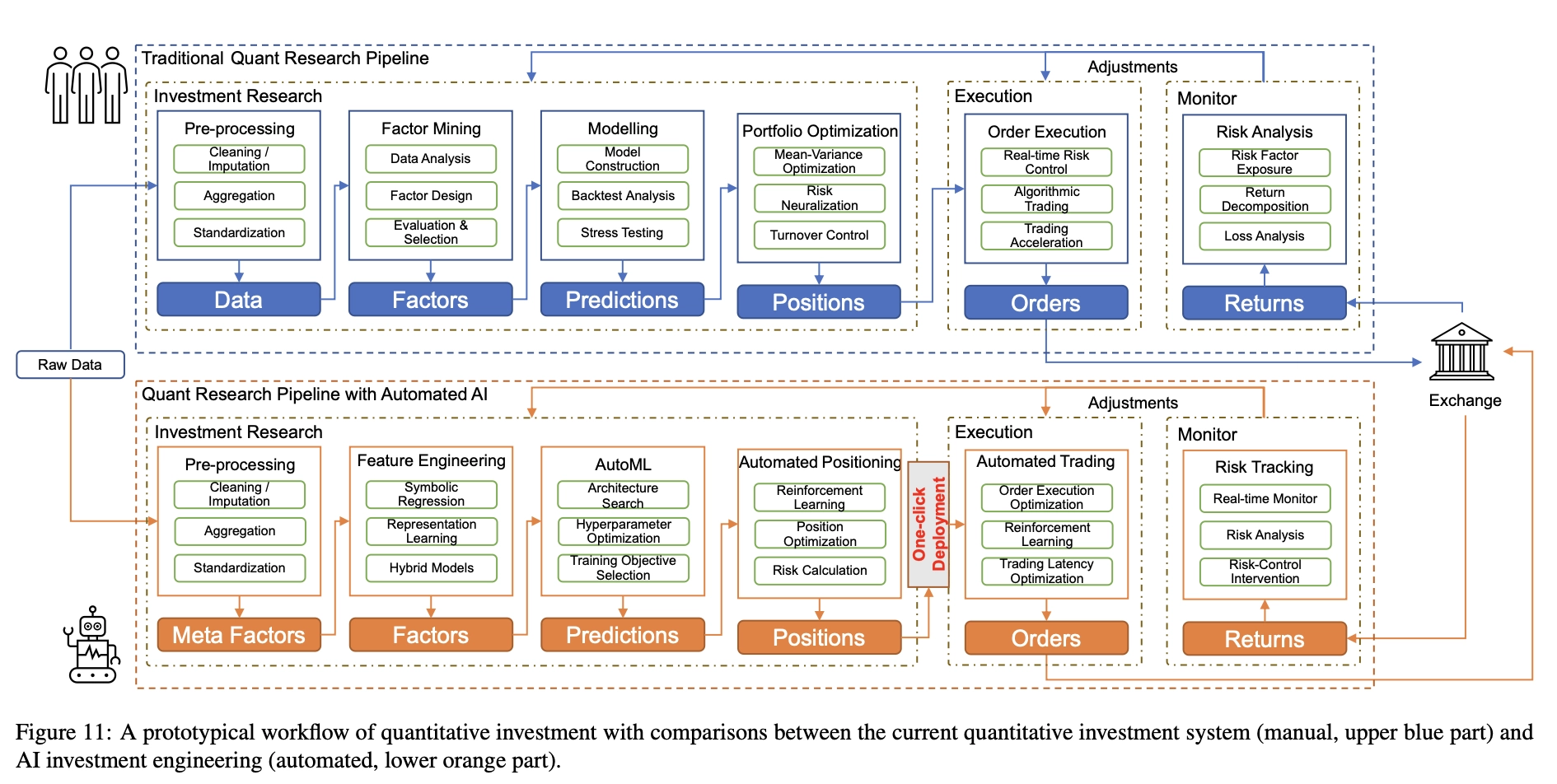
The automated process of Quant 4.0 is shown in Figure 11 (orange part), in which the modules in the process are automated by applying the most advanced artificial intelligence technology. In the remainder of this section, we will focus on the three core modules in the automation process.

1. Automatic Factor Mining: Apply automated feature engineering techniques to search and evaluate important financial factors generated from meta-factors. We will introduce popular search algorithms and demonstrate how to design algorithmic workflows.
2. Automatic modeling: Apply AutoML technology to discover the optimal deep learning model, automatically select the most appropriate model and the best model structure, and adjust the best hyperparameters.
3. One-click deployment: Build an automated workflow to deploy large-scale trained models on trading servers with limited computing resources. It automatically performs model compression, task scheduling and model parallelization, saving a lot of manpower and time from tedious “dirty work”.

Automated factor mining

For feature engineering in the quantitative field, it refers to the process of extracting financial factors from raw data. Due to its inherent noise characteristics, these data are difficult to perform effective pattern recognition [49, 50, 51]. Traditionally, financial factors with significant “alpha” have been manually explored and developed by quantitative researchers, who rely on expert domain knowledge and comprehensive understanding of financial markets. Although some financial institutions are beginning to use random search or general-purpose programming algorithms, these techniques are primarily used as small-scale aids to help make quantitative researchers more productive. In Quant 4.0, we propose to automate the factor mining process, formulate feature engineering as a search problem, and utilize corresponding algorithms to generate factors with satisfactory backtest performance at scale. According to their expression form, we classify factors into

1. Symbolic [52] factors, these are symbolic equations or symbolic rules
2. Machine learning factors, these are represented by neural networks, which we will elaborate on in the following sections.

Sign factor

Symbolic factor mining can be viewed as a special case of symbolic regression [56]. Traditional symbolic regression algorithms typically generate a large number of symbolic expressions from given operands and operators and select the symbolic expression that maximizes a predefined objective function. Figure 12 shows the framework of automated symbolic factor mining, which includes four core parts: operand space, operator space, search algorithm and evaluation criteria.

• operand space: defines which meta-factors can be used for factor mining. Meta-factors are the basic components of factor construction. Typical meta-factors include basic price and trading volume information, industry classification, basic features extracted from limit/order books, common technical indicators, basic statistical data from financial analysts, announcements from public companies, financial reports and other research reports, emotional signals of investor sentiment [57, 58], etc.

• Operator Space: Defines which operators can be used during factor mining. For example, in cross-sectional stock selection, operators can be divided into primary operators for constructing symbolic factors and post-processing operators for normalizing factors in different trading environments. The main operators can be further classified into element-wise operators such as () and log(), time series operators such as ts rank() and ts mean(), which calculate the rank and mean of each stock respectively, cross-sectional operators such as rank() and quantile(), which calculate the rank and quantile along a cross-section at a specific trading time, and group operators such as group rank(), which calculate the rank in each group (such as industry or sector) respectively. Post-processing operators are used to “fine-tune” the resulting factors. Typical post-processing operators include winsorization [43] to clip outliers and normalization operators to unify the data range, neutralization operators for risk balancing, grouping operators to limit the stock selection range, and decay operators to control turnover rates and thereby reduce transaction costs.

• Search Algorithm: The search algorithm is designed to search and find valid or qualified factors in the most efficient way possible. A simple way to generate new factors is the Monte Carlo (MC) algorithm, which randomly selects elements in the operand and operator space and recursively generates a symbolic expression tree. Unfortunately, as the length and complexity of the generated formulas increase, the search time can grow exponentially, forcing us to consider more efficient alternatives. The first choice is the Markov Chain Monte Carlo (MCMC) algorithm [59], which generates factors from the posterior distribution in an importance sampling manner and is therefore more efficient than MC. The second option is genetic programming [61], a special evolutionary algorithm for sampling and optimizing tree-like data. A third option involves gradient-based methods, such as neural networks, which approximate discrete symbolic formulas with continuous nonlinear functions and search along the gradient direction, significantly more efficiently than random search.

• Evaluation Criteria: Evaluation criteria are used to measure the quality of factors found by the search algorithm. Evaluate the performance of generated factors through backtesting experiments. Typical evaluation criteria include information coefficient (IC), information ratio based on information coefficient (ICIR), as well as annualized return, maximum drawdown, Sharpe ratio and turnover rate. In addition, it is very important to maintain the information diversity among factors by filtering redundant factors that are highly correlated with other factors.

Machine learning factors

Symbolic factors are widely used in practice because of their simplicity and understandability. However, their representational capabilities are limited by the richness of operands and operators. On the other hand, machine learning factors are more flexible in their representation to accommodate more complex nonlinear relationships [67], so they have the opportunity to perform better in market predictions. In particular, mining machine learning factors [68, 69, 70, 71] is a process of fitting neural networks where gradients provide optimal directions for a fast search for solutions. As shown in Figure 15, most deep neural networks for stock prediction follow an encoder-decoder architecture [72], where the encoder maps meta-factors to latent vector representations and the decoder converts this embedding into some outcome, such as future returns [73]. In fact, not only the final results, but also the embeddings themselves can be used as (high-dimensional) machine learning factors [74] and further applied to various downstream tasks.

Machine learning factors also have some limitations. First, due to the black-box nature of machine learning, they are often difficult to interpret and understand. Second, the gradient search used by neural networks may get stuck in some local optima and lead to model instability issues. Finally, due to their flexibility, neural networks may be more susceptible to overfitting, and in the quantitative domain, the situation becomes even more severe because the data is extremely noisy.

Whether it is automatically mining symbolic factors or directly fitting machine learning factors, they are purely data-driven methods. To succeed in extremely low signal-to-noise ratio financial data, a large amount of prior knowledge needs to be manually introduced.

Automated modeling

Automation of statistical machine learning, such as support vector machines (SVM), decision trees, and boosting, has been extensively studied. A simple and straightforward approach to automation is to enumerate all possible configurations, including the choice of machine learning algorithms and corresponding hyperparameters. In this paper, we focus on the state-of-the-art deep learning automation problem, which is further complicated by the end-to-end nature and network architecture issues in modeling. The configuration of a deep learning model consists of three parts: architecture, hyperparameters, and goals, which together determine the final performance of the model. Traditionally, these configurations have been manually adjusted. In Quant 4.0, they are searched and optimized through various AutoML algorithms. A standard AutoML system needs to answer the following three questions: what to search (i.e., search space), how to search (i.e., search algorithm), and why to search (i.e., performance evaluation).

Search space

The search space is designed for three configuration settings that need to be optimized in an automated manner.

• Architecture Configures the network structure. For example, the architecture of a multilayer perceptron is specified by the number of hidden layers and the number of neurons in each layer. The architecture of a convolutional neural network needs to consider more configurations, such as the number of convolution kernels and their strides and receptive fields. The architecture of large-scale models (such as Transformer) consists of many predefined blocks (e.g., self-attention blocks, residual blocks). As mentioned above, architectures are complex and may have hierarchical structures at different scales. Therefore, the search space can be defined at different granularities, from low-level operators such as convolution and attention to high-level modules such as LSTM units. Early search algorithms operated at the finest granularity and optimized the low-level structure of neural networks. Such a search process is flexible in network structure but less efficient in integrating prior knowledge and abstraction. One solution is to assume a layered structure in the network architecture. Specifically, at a high level, networks are designed as graphs of cells (i.e., blocks/topics [42, 80]), with each cell being a subnetwork. To reduce computational costs, many cells share the same internal structure at a low level. Cell-based search algorithms [81, 82] need to find high-level structures between cells as well as low-level structures within cells.

• Hyperparameters control the entire training process. For example, the learning rate determines the step size toward the minimum value of the loss function. Smaller learning rates result in more accurate solutions, but slower convergence. Batch size determines the number of samples involved in the batch used for gradient estimation, which also affects the efficiency and stability of training. Compared to the search space of the architecture, the search space of hyperparameters is simpler because most hyperparameters are continuous (e.g., learning rate) or approximately continuous (e.g., batch size).

• Target specifies the loss function and labels used during training. The loss function is a key component of a machine learning model because it provides the target to which the model should be trained. In addition to classic loss functions such as mean square loss and cross-entropy loss, it is also possible to choose new loss functions designed specifically for quantization tasks. The label defines the “ground-truth” target that the model aims to fit. For example, price increases and decreases or future returns over different holding time windows can be considered in the search space.

The difficulty of selecting/designing loss functions in the field of asset pricing is beyond imagination. The optimization goal of traditional machine learning algorithms is to minimize the model’s single-sample prediction error. In practice, the Sharpe ratio of the portfolio is examined. The covariance of the prediction error is equally important as the mean. Not only that, compared with general tasks, the number of labels for quantitative stock selection is not only small, but also mostly composed of noise. Simply applying the existing loss function is not consistent with the performance of the investment portfolio within the sample, let alone out of the sample. At this point, a breakthrough in financial theory is urgently needed, and automated machine learning technology is powerless.

Search algorithm

We can use a search algorithm to find the optimal model configuration given a search space. Table 2 lists various types of search algorithms and their corresponding tasks: Network Architecture Search (NAS) [75], Hyperparameter Optimization (HPO) [83] and Training Target Selection (TOS). Grid search is a brute force algorithm that searches over a grid of configurations and evaluates all configurations within it. Due to the simplicity of implementation and parallelization, it is a good choice when the search space is small [84]. However, most NAS and HPO problems in deep learning have extremely large search spaces, and grid search does not scale well to these problems. In addition, grid search is more commonly used in HPO and TOS than in NAS because the search space of NAS is difficult to grid layout except enumerating all possibilities.

• Random Search Generates several candidate configurations using some random sampling mechanism (such as Monte Carlo or MCMC). It is very intuitive to understand and easy to implement and parallelize (mainly used for independent sampling mechanisms such as Monte Carlo sampling or importance sampling). Random search is very flexible and can be used on NAS, HPO and TOS. Although random search is generally faster than grid search [84], it is still difficult when dealing with high-dimensional search spaces because the number of potential configurations grows exponentially with the number of hyperparameters.

• Evolutionary Algorithm is an extension of random search. It utilizes evolutionary mechanisms to iteratively improve model configurations. It encodes the network architecture as a population and performs evolutionary steps on it to iteratively improve the model. Specifically, the model is first encoded according to its underlying computational graph. A set of predefined evolution operations are then applied to the encoded model, including structural modifications such as inserting or deleting multiple operations and adding skip connections, as well as hyperparameter-related operations such as learning rate adjustments. In each iteration, the best-performing models are selected through a tournament and combined through mutation and crossover operations to form the next generation. Evolutionary algorithms inherently support weight inheritance between generations, helping to accelerate training convergence and improve search efficiency.

• Bayesian Optimization explores the search space of objective functions that cannot be explicitly expressed more efficiently by leveraging surrogate models. Specifically, for the black-box objective function of HPO, Bayesian optimization uses a surrogate function (such as a Gaussian process or a tree-like Parzen estimator) to initialize the prior distribution. New data points are then sampled from the prior distribution (with significance) and their values ​​are calculated using the underlying objective function. Given these new samples and a prior, a posterior function can be calculated and used as an updated surrogate function in place of the original prior function. This process is repeated until the optimal solution is found. Traditionally, Bayesian optimization has been used for continuous search tasks such as HPO, but recent research has extended it to NAS tasks as well.

• Gradient-based methods are very efficient when the gradient of the objective function exists. However, for NAS, the search space is discrete and the gradient cannot be defined directly. One solution is to “soften” the architecture and define a hyperparameterized “hyperarchitecture” that covers all possible candidates and is differentiable. A typical gradient-based NAS method is DARTS [97], which constructs a hyperparameterized network in which all types of candidate operations are included on the computational graph. The result value is the weighted sum of the results of all operations, where the weights are the softmax values ​​of the parameterized probability vector. Through a two-layer optimization problem, model parameters and architecture parameters are trained. During inference, the architecture and hyperparameters with the highest probability are selected. On NAS and HPO tasks, DARTS is much faster than random search and reinforcement learning.

Automated complex model design is exciting, but while improving in-sample prediction performance, we must also consider the risk of backtest overfitting

Accelerate evaluation

The computational cost of automated model search comes from two parts: the search algorithm and model evaluation, with the latter often being the computational bottleneck because training a deep neural network until convergence under a given configuration is time-consuming. Several methods have been introduced in previous studies to address this issue. First, the training process of the neural network can be stopped early before convergence to reduce the computational time of the evaluation [81]. Secondly, the model can select fewer samples to speed up the training process [94]. Third, hot-start model training can be used to exploit information from a selected model [102], or to inherit information from a hyperparameterized “parent” model [103, 97, 98] to speed up the search loop.

Automated deployment

Model deployment is the task of transferring developed models from offline research to online trading. This involves not just the transfer of code and data, but also synchronization of data and factor dependencies, adapting trading servers and systems, debugging model inference, testing computational latency, and more. In the following sections, we focus on an important issue in model deployment: how to accelerate deep learning inference for high-frequency trading and algorithmic trading scenarios. We propose an automated one-click deployment solution that leverages technologies such as model compilation [104] and model compression [105, 106] to achieve inference acceleration [104, 105, 106]. The former makes inference faster without changing the model itself, and the latter looks for smaller, lighter alternative models to save inference time.

Model compilation acceleration

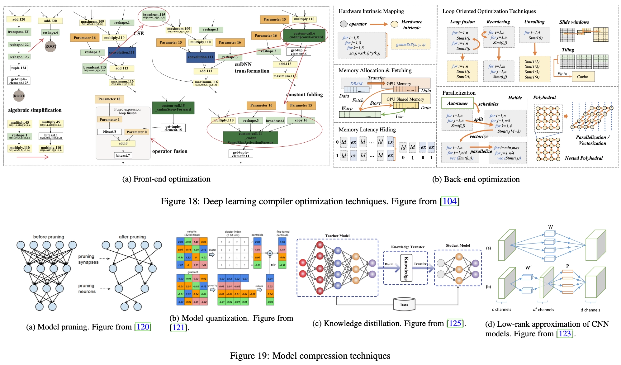
During the development phase, the functionality of the deep learning model is the first priority to implement the underlying framework for computing. Therefore, at this stage, the framework strictly maps all operations into the computational graph. However, this direct mapping introduces a large amount of optimization space in the deployment phase where the calculation is fixed. Therefore, the computation of the model can be greatly simplified and adapted to the hardware characteristics without compromising its original semantics. This optimization is one of the main topics in deep learning compilers [107, 108, 109] and can be divided into front-end optimization and back-end optimization, which work on high-level and low-level intermediate representations (IRs) of deep learning models, respectively. Following the summary of [104], we will briefly introduce related optimization techniques.

Front-end optimization, shown in Figure 18a, focuses on simplifying the structure of the computational graph. For example, algebraic simplification techniques such as constant folding [110] and intensity reduction [111] convert expensive operations into cheap operations through transformations or merging. Common Subexpression Extraction (CSE) [112] technique identifies duplicate nodes in the computation graph and merges them into a single node to avoid duplicate computations.

Backend optimization, shown in Figure 18b, focuses on the characteristics of the hardware architecture, such as locality and memory latency. For example, prefetching techniques [113] load data from main memory to the GPU and then speed them up before they are needed. Loop-based optimization [114] rearranges, fuses, and unrolls operations inside loops to enhance locality between adjacent instructions. Memory latency hiding [115] technology aims to improve instruction throughput to alleviate high latency issues when accessing memory. Parallelization techniques, such as loop splitting [116], auto-vectorization [117] and loop skewing [118, 119], can also be applied to maximize the use of the parallelism offered by modern processors.

Model compression acceleration

The goal of model compression is to reduce model size at inference time while reducing performance degradation. In this way, the compressed model can be viewed as an approximation of the original model. Generally speaking, model compression can be performed at both micro and macro levels, with the former focusing on the accuracy of individual model parameters and the latter focusing on simplifying the overall model structure.

At the micro level, pruning and quantization techniques can be applied to reduce the number of parameters and the number of bits in a single parameter. Model pruning [120], as shown in Figure 19a, removes unimportant connections and neurons that have little impact on the activation of neurons in the neural network. The identification of candidate parameters is usually based on their weights, where parameters with smaller weights are considered for pruning. Model quantization [121], as shown in Figure 19b, converts parameters from floating point numbers to low-bit representation. Specifically, a codebook is constructed that stores approximations of the original parameters based on the distribution of all parameter values. Then, the parameters are quantized according to the codebook, thereby reducing the number of bits in the parameters. Since performance degradation caused by reduced accuracy is inevitable, compressed models are often retrained to get closer to their original performance.

At the macro level, the model can be significantly compressed into a smaller model with a simpler architecture through techniques such as knowledge distillation [122] and low-rank decomposition [123, 124]. Knowledge distillation (Figure 19c) compresses the model by transferring useful knowledge from the original large model (called the teacher model) to a small and simple model (called the student model), minimizing knowledge loss. The low-rank decomposition technique (Fig. 19d) assumes the sparsity of the model parameters, and then decomposes the parameter matrix of the original neural network into the dot product of the low-rank matrix, thereby reducing model complexity.

Deep learning model compilation and compression technology is an important general optimization technology for deploying deep learning models. However, usually, quantitative trading is not a task with high request volume, and model reasoning is not stuck or difficult. Therefore, investing in performance optimization that reduces model accuracy may not be worth the gain.