Quant 4.0 (I): An Introduction to Quantitative Investment, from 1.0 to 4.0

Chinese

In recent years, the quantitative investment industry has been booming in China and has become an unavoidable topic when discussing the secondary market. It is either mythical or criticized by everyone. So, what exactly is quantitative investment (Quantitative Investment)? What quantitative strategies are there? Are quantitative strategies guaranteed to make money? What are the basic principles for building a quantitative strategy? This article introduces the basic concepts of quantitative investment, its past and present, and looks forward to its future development model.

This article is a partial translation of the paper Quant 4.0: Engineering Quantitative Investment with Automated, Explainable and Knowledge-driven Artificial Intelligence, with some deletions. Original address

Quant4.0 (1) Introduction to quantitative investment, from 1.0 to 4.0

Quant4.0 (2) Automated AI and Quantitative Investment Research

Quant4.0 (3) Explainable AI, knowledge-driven AI and quantitative investment research

Quant4.0 (4) System integration and simplified version of quantitative multi-factor system design

Wealth Management and Quantification

The wealth management industry is one of the largest sectors of the global economy. According to a global wealth report[1] by the Boston Consulting Group (BCG), the scale of global financial wealth has increased from US\(188.6 trillion in 2016 to US\)274.4 trillion in 2021, which is almost three times the global nominal gross domestic product in 2021. Additionally, the company predicts this number will increase to $355 trillion by 2026. With the rapid development of the digital economy, big data and artificial intelligence, more and more new technologies are applied to the wealth management industry, leading to a branch of financial technology/engineering called “investment engineering” [3]. The processes of investment research, trade execution, and risk management are becoming systematic, automated, and intelligent, a concept that has been implemented in the recent evolution of quantification.

As an important group of participants in the financial market and wealth management industry, quantitative investment now uses rigorous mathematical and statistical modeling techniques, machine learning techniques, and algorithmic trading techniques to discover asset pricing anomalies in the financial market and profit from subsequent arbitrage or investment opportunities. Quantitative investing has many advantages over traditional fundamental and technical investing.

• First, the performance of quantitative strategies can be pre-checked and evaluated using backtest experiments based on historical data before real trading begins.
• Second, quantitative trading has a speed advantage in quoting orders at the best price.
• Third, it removes the negative impact of human emotions from the decision-making process. Finally, in terms of data analysis, quantitative research has significant advantages in the depth, breadth and diversity of financial market and industry information.

In the past 30 years, information infrastructure and computer technology have been widely used in the global financial trading market. Today, vast amounts of financial data are generated every second and millions of orders are executed, leading to rapid growth in the quant industry. Taking the U.S. stock market as an example, more than 60% of the total trading volume comes from computer trading algorithms rather than human traders.

Quantitative strategy

Quantitative strategy is a system that makes trading decisions based on predefined rules or trained models. It is usually the core intelligent asset of quantitative funds.

Components of quantitative strategies

A standard quantitative strategy consists of a series of components such as investment instruments, trading frequency, trading patterns, strategy types and data types.

• Investment Instruments specifies which financial instruments the strategy includes for investment. Popular candidate instruments include stocks, exchange-traded funds (ETFs), bonds, foreign exchange, convertible bonds, and more complex financial derivatives such as futures, options, swaps, and forwards [6]. Investment strategies can trade a single type of instrument (for example, a strategy for trading ETFs) or multiple types of instruments (for example, an alpha hedging strategy that is simultaneously long stocks and short index futures to eliminate market risk).
• Trading Frequency specifies how assets in the portfolio are held and how frequently they are traded. Typically, high-frequency trading holds positions over minutes or seconds, while low-frequency trading may hold assets over months or years. The significant difference in holding periods leads to very different considerations in strategy design compared to high-frequency trading and low-frequency trading. For example, for high-frequency trading, asset capacity limitations and transaction costs are significant issues, while for low-frequency trading, we should carefully think about how to control drawdown risks [7].
• Model Type characterizes how the trading problem is formally modeled. Examples include cross-sectional trading, time series trading, and event-driven trading[7]. Cross-sectional trading is commonly used in stock selection, where all stocks in a quantitative strategy are ranked by the score of future returns predicted by the model. The portfolio manager can go long the stocks with the highest scores and short the stocks with the lowest scores. Unlike time series trading, event-driven trading has intervals that are unevenly distributed in time, where investment decisions and trade executions are triggered by the occurrence of events.
• Trade Types are a series of thinking templates for how we design our strategies. Examples include momentum trading [8], mean reversion trading [9], arbitrage trading [10], hedging [11], market making [12], etc. By utilizing these strategy types, traders can explore profit opportunities from different aspects of the financial markets. Specifically, momentum trading assumes that the price trend is sustainable over the following time window and trades in the direction of this trend. In contrast, a mean reversion trade bets that the price trend will move in the opposite direction in the near future and takes a position in the opposite direction. Hedging is the purchase of one asset to reduce the risk of loss in another asset. Arbitrage is the simultaneous longing and shorting of the same asset in different markets, or the longing and shorting of a pair of highly correlated assets to profit from the convergence of price differences. Market making is a transaction that provides liquidity, quoting buy and sell prices for tradable assets in the hope of profiting from the bid-ask spread.
• Data Type indicates what type of data is used in the policy. Typical data types include market data, limit order books [13], news data, financial statements, analyst reports, as well as alternative data such as sentiment data, location data, and satellite images. During the strategy development process, strategy researchers must consider what data they have and what data they need during the strategy development process. For example, limit order book flows are often used to build high-frequency trading strategies, while news data is more commonly used in event-driven strategies.

Basic principles of asset management

Similar to how learning the law of conservation of energy can help avoid falling into the trap of perpetual motion, learning some basic principles of asset management can be beneficial to escape some common pitfalls in strategy development.

Basic Laws of Active Management

The first principle is the fundamental law of active management proposed by Richard Grinold and Ronald Kahn [15]. This law states that the performance of an active investment manager (or equivalent quantitative model) depends on the quality of investment skills and the number of investment opportunities. This law can be expressed mathematically as:

$$\text{IR} = \text{IC} \times \sqrt{\text{BR}},$$

Among them:

• \(\text{IR}\) represents the information ratio, which measures the effect of active management;
• \(\text{IC}\) represents the information coefficient, which is the accuracy of the model’s prediction of future returns;
• \(\text{BR}\) represents the ratio of the frequency of investment opportunities to the observation time window.

This formula emphasizes that the key to active management lies in the quality of investment skills and the frequency of investment opportunities. If an investment manager can predict future returns more accurately (higher information coefficient) and has more investment opportunities, then its active management results will be better. This is an important principle for developers of quantitative strategies as it guides their efforts to improve the accuracy of model predictions and find more investment opportunities. When assessing investment quality, breadth represents the number of independent investment decisions made in a year, while IR is the ratio of portfolio returns over benchmark returns to return volatility, a measure of asset management performance. Mathematically, the fundamental laws of active management can be viewed as an application of the central limit theorem in mathematical statistics [16]. When applying this rule in practice, we must note that IC and breadth are usually not independent. For example, given a strategy, we can increase its breadth by relaxing the threshold for trading signals, but in doing so, the IC may decrease because more false positive noise is introduced into our decisions. Therefore, a good strategy should find an optimal trade-off between these two coupling variables. Figure 4a shows the distribution of various popular strategies in terms of IC and breadth, as well as their corresponding IR performance.

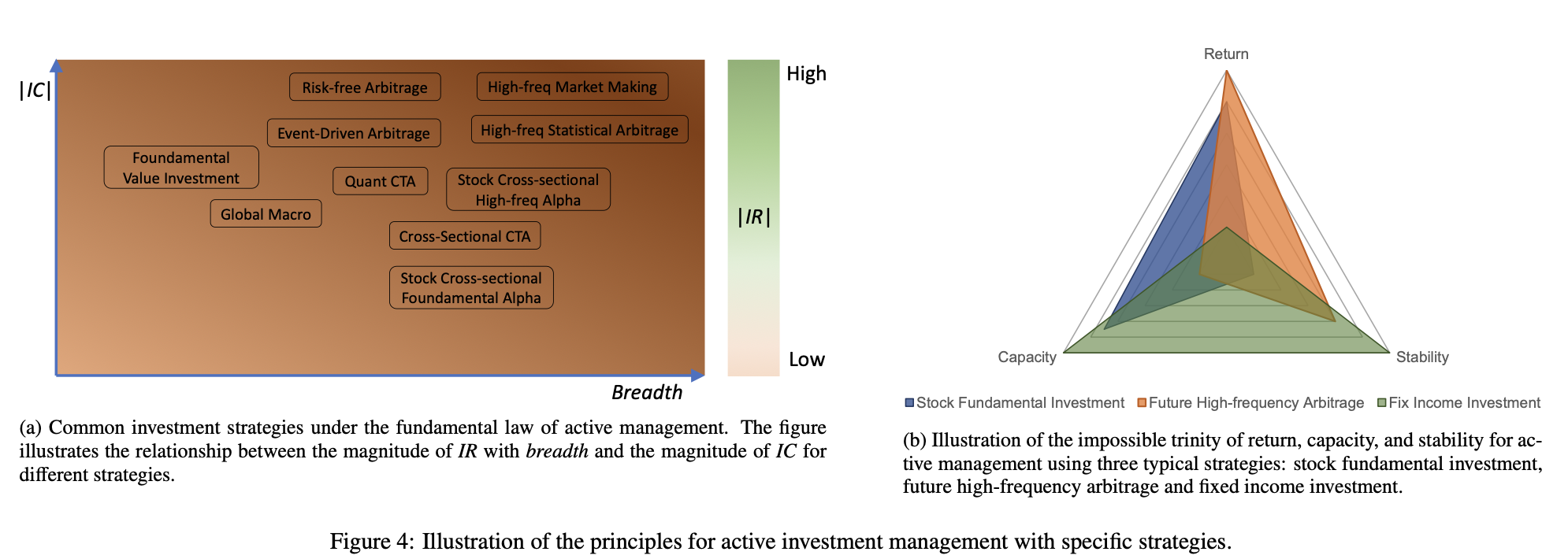
The figure above shows the distribution of various strategies in information coefficient (IC) and breadth, as well as their corresponding information ratio (IR) performance. The horizontal axis represents IC, the vertical axis represents breadth, and points of different colors and shapes represent different strategies. It can be seen that some strategies perform well in IC but have low breadth, while other strategies perform well in breadth but have relatively low IC. The dotted traces in the figure represent the contours of different IR values, which indicate the range of IR values ​​in the space of IC and breadth. As can be seen from this figure, the optimal strategy usually finds a balance between IC and breadth to maximize IR.

The Impossible Triangle of Investment

The second principle is the Impossible Triangle of Asset Management. Specifically, no investment strategy can satisfy the following three conditions at the same time, namely high return, low risk (or equivalently high stability) and high capacity. Figure 4b uses a radar chart to illustrate the Impossible Triangle, which includes three variables: return, stability, and capacity. For example, high-frequency market making and calendar arbitrage strategies may be able to achieve high returns and stability (low portfolio volatility), but their AUM capacity is typically small, often exceeding billions of dollars even in global transactions. In contrast, equity fundamental strategies have high capacity, reaching trillions of dollars, but their returns and stability are not as good as high-frequency trading. The chart above illustrates the Impossible Triangle of investing through a radar chart, which includes three key variables: return, stability, and capacity. Different colored areas represent different investment strategies. It can be clearly seen that no strategy can achieve optimal performance in these three aspects at the same time. Investors need to find a balance between the three and choose the appropriate strategy based on their risk appetite and goals.

The history of quantitative investing

The origins of quantitative investing can be traced back to more than a century ago, when French mathematician Louis Bachelier published his doctoral thesis “The Theory of Speculation” in 1900 [17], which showed how to use the laws of probability and mathematical tools to study stock price movements. As the first pioneer to explore the application of advanced mathematics to financial markets, Bachelier’s work inspired the rise of academic research in quantitative finance, although it was not widely used in actual industry due to the scarcity of data at the time. Quantitative investing was first practiced by American mathematics professor Edward Thorp, who used probability theory and statistical analysis to win the game of blackjack and subsequently applied his research to seek systematic and stable returns in the stock market [18]. In this subsection, we introduce the history and milestones of the development of quantitative finance from two aspects: research milestones in academia and the evolution of quantitative investment in actual industry practice.

Q-Quant and P-Quant

Academia and the investment industry divide quantitative finance into two branches, often referred to as “Q-Quant” and “P-Quant.” These two branches are modeled based on risk-neutral measures and probabilistic measures respectively, hence the name. Generally speaking, Q-Quant studies derivatives pricing issues and extrapolates the current situation, using a model-driven research framework. Data are usually used to adjust the parameters of the model. P-Quant, on the other hand, studies quantitative risk and portfolio management, modeling the future, using a data-driven research framework, and building different models to improve fitting of historical data. Typically, Q-Quant research is conducted among sell-side institutions (such as investment banks and securities firms), while P-Quant is more popular among buy-side institutions (such as mutual funds and hedge funds). Table 1 compares the characteristics of these two types of quantification.

Table 1: Comparison between P-Quant and Q-Quant [19]

Type	Goal	Scenario	Measurement	Modeling	Example	Algorithm	Challenge	Business
Q-Quant	Extrapolate Current	Derivatives Pricing	Risk Neutral Measures	Continuous Stochastic Processes	Black-Scholes Model	Ito Calculus, PDE	Calibration	Sell Side
P-Quant	Simulating the future	Portfolio management	Probability measures	Discrete time series	Multi-factor models	Statistics, machine learning	Estimation/forecasting	Buy-side

Milestones for Q-Quant

In 1965, Paul Samuelson, an American economist and winner of the 1970 Nobel Prize in Economics, introduced stochastic processes and stochastic calculus tools to analyze financial markets and model stochastic changes in stock prices [20]. In the same year, he published a paper on the life cycle portfolio selection problem, using stochastic programming methods [21]. In the same year, another American economist, Robert Merton, also published his work on life cycle portfolio selection. Unlike Samuelson’s approach using discrete-time stochastic processes, Merton’s work used continuous-time stochastic calculus to model the stochastic uncertainty of portfolios [22]. Almost in the same year, economists Fischer Black and Myron Scholes proved that the expected returns and risks of asset management could be eliminated by dynamically adjusting the portfolio, and therefore invented the risk-neutral strategy of derivatives investment [23]. They applied this theory to actual market transactions and published it in 1973. This risk-neutral model was later named after them and became known as the Black-Scholes model [24], a partial differential equation (PDE) tool used to price financial markets containing derivative investment instruments. Specifically, the Black–Scholes model establishes a partial differential equation that controls the evolution of the European option call or European option put price, as follows:

$$ \frac{\partial V}{\partial t} + \frac{1}{2} \sigma^2 S^2 \frac{\partial^2 V}{\partial S^2} + rS \frac{\partial V}{\partial S} - rV = 0 $$

where V is the option price as a function of the stock price S and time t, r is the risk-free rate, and σ is the stock’s volatility. This partial differential equation has a closed solution, known as the Black-Scholes formula. Since Robert Merton was the first to publish a paper that expanded the mathematical understanding of option pricing models, he is often credited with his contribution to this theory. Merton and Shores won the 1997 Nobel Prize in Economics for their discovery of risk-neutral dynamic revision. Later, the original Black-Scholes model was extended to accommodate deterministic variable interest rates and volatilities and was further used to characterize European option prices for dividend-paying instruments, as well as American and binary options.

As a pioneering work in risk-neutral theory, one of the many limitations of the Black-Scholes model is the assumption that the underlying volatility is constant over the term of the derivative and is not subject to changes in the price level of the underlying security. This assumption is often contradicted by the smiling curve and skewed shape phenomena of the implied volatility surface. Relaxing the constant volatility assumption is a possible solution. Modeling derivatives can be practiced more accurately by using stochastic processes to characterize the volatility of underlying prices, and this idea led to a series of works on stochastic volatility, such as the Heston model [25] and the SABR model [26]. As a commonly used stochastic volatility model, the Heston model assumes that changes in the volatility process are proportional to the square root of the variance itself and exhibit a tendency to revert to the long-term mean of the variance. Another commonly used stochastic volatility model is the SABR model, which is widely used in the interest rate derivatives market. The model uses stochastic differential equations to describe a single forward (such as a LIBOR forward rate, a forward swap rate, or a forward stock price) and its volatility, and has the ability to reproduce the volatility smile curve effect. In recent years, deep learning and reinforcement learning techniques have been applied in combination with risk-neutral Q-Quant modeling. Hans Buehler introduced the concept of learning trading and proposed the deep hedging model [27], which is a framework for hedging derivatives portfolios in the presence of market frictions (such as transaction costs, market impacts, liquidity constraints, or risk constraints) and uses deep reinforcement learning and market simulation to model the volatility stochastic process. It no longer uses formulas but naturally captures the co-movements of relevant market parameters.

In addition to derivatives pricing models, market efficiency theory and risk modeling theory are also very important in Q-quant, both in academia and industry. In the 1980s, Harrison and Pliska established the Fundamental Theorem of Asset Pricing [28], which provided a series of necessary and sufficient conditions for an efficient market without arbitrage and a complete market. In 2000, David The Gaussian Copula has quickly become a tool used by financial institutions to correlate relationships between multiple financial securities because it is relatively simple to model even for complex assets that were previously difficult to price, such as mortgages.

Milestones of P-Quant

Q-quant plays an extremely important role in quantitative finance. However, in this article, we stand from the buyer’s perspective and focus on asset prediction and portfolio optimization problems. Therefore, unless otherwise stated, all the following discussions about quantitative investment are based on the P-quant perspective.

The origins of P-quant begin with the establishment of modern portfolio theory, introduced by Harry Markowitz. The theory was first proposed in his doctoral thesis “Portfolio Selection” and published in the Journal of Finance in 1952 [31], and later expanded in his 1959 book “Portfolio Selection: Efficient Diversification of Investments” [32]. Following the old adage “Don’t put all your eggs in one basket,” Markowitz developed the concept of the efficient frontier for asset investment in financial markets and maximized the expected return of a portfolio at a certain level (usually measured by the variance of the assets in the portfolio) by mathematically formulating it as a quadratic optimization problem.

Based on modern portfolio theory, the capital asset pricing model (CAPM) was subsequently independently proposed by Jack Treynor (1961, 1962) [33], William F. Sharpe (1964) [34], John Lintner (1965) [35] and Jan Mossin (1966) [36]. The goal of CAPM is to describe the relationship between the market’s systematic risk and the expected return of an asset.

$$E(R_p) - R_f = \alpha + \beta \cdot (E(R_m) - R_f)$$

Where \(E(R_p)\) is the expected return of the investment portfolio, \(R_f\) is the risk-free return, and \(E(R_m)\) is the expected return of the market. Specifically, CAPM breaks down asset return and risk into two separate components, alpha and beta. Alpha measures the performance of a portfolio relative to a benchmark index (such as the S&P 500 Index), while beta measures the variance of a portfolio relative to the benchmark index and represents the risk caused by market fluctuations. One of the major contributors to CAPM, William Sharp, shared the 1990 Nobel Prize with Harry Markowitz. Another important step in quantitative finance was the Arbitrage Pricing Theory (APT) proposed by MIT economist Stephen Ross in 1976. APT improves on its predecessor, CAPM, by further introducing a multi-factor model framework to establish the relationship between asset prices and various macroeconomic risk variables. Within the framework of the multi-factor model, Nobel Prize winner Eugene Fama and his colleague Kenneth French from the University of Chicago jointly proposed the famous Fama-French three-factor model in 1992.

$$E(R_p) - R_f = \beta_0 + \beta_1 \cdot (E(R_m) - R_f) + \beta_2 \cdot SMB + \beta_3 \cdot HML$$

The model relates expected portfolio return (minus the expected value of the risk-free return) to three systematic risk factors: expected market return \(E(R_m) - R_f\), size \(SMB\) (the difference between small-cap stocks versus large-cap stocks), and book-to-market ratio \(HML\) (the difference between high-book-to-market versus low-book-to-market firms). The three-factor model was subsequently expanded into the Fama and French five-factor model in 2015, adding two factors: profitability (the difference in returns between the most and least profitable companies) and investment riskiness (the difference in returns between conservative and aggressive investment companies).

Parallel to advances in multifactor models, the 1980s saw the emergence of many important studies on time series analysis. In 1980, Nobel Prize winner Christopher Sims introduced the vector autoregressive (VAR) model to the fields of economics and finance. As an extension of the single-series autoregressive (AR) model and the autoregressive moving average (ARMA) model commonly used in time series analysis, VAR characterizes the autoregressive properties between multiple time series over time and assumes that the variance of the error term in the regression formula is constant. In 1982, Robert Engler introduced the autoregressive conditional heteroscedasticity (ARCH) model and extended it into the generalized autoregressive conditional heteroscedasticity (GARCH) model to characterize financial fluctuation patterns in the market by specifying random variance in the model. In 1987, he jointly introduced the cointegration method with Clive Granger (the discoverer of Granger causality, which is used to model lead-lag patterns between multiple time series) to test the significance of mean reversion patterns in financial time series. The cointegration test has been widely used to discover promising asset pairs for statistical arbitrage strategies. Engler and Granger shared the Nobel Prize in 2003 for their contributions to time series analysis, which is used in quantitative finance for market forecasting and investment research.

In 2018, three pioneers of deep learning technology, Yoshua Bengio, Geoffrey Hinton and Yann LeCun, won the Turing Award. Today, deep learning has been widely used in the financial field by academic researchers. Quantitative researchers in financial institutions use deep learning to build complex nonlinear models to learn the relationship between financial signals and expected returns, and to predict asset prices. Its powerful ability in fitting big data has significantly improved the performance of market forecasts and portfolio management.

Although accurately predicting the future trend of asset prices is a very important task in P-Quant, quantitative researchers are more concerned with how to explain the effect of model predictions and explain the way the model really works, because in the risk management of portfolio managers, “why” is more critical than “what”. Causal effect analysis [39] and factor importance analysis are two core tasks in quantitative model interpretation. Clive Granger invented the Granger causality test in 1969 [40] to determine whether one time series is useful in predicting another time series. Although there is controversy over whether the Granger causality test is capable of statistically assessing “true” causal relationships, the method has been widely used in quantitative research, such as searching for and evaluating stock pairs with significant lead-lag effects and trading them with corresponding strategies. In 1994, Guido Imbens and Joshua Angrist, who jointly won the Nobel Prize in Economic Sciences in 2021, introduced the local average treatment effect (LATE) model to characterize statistical causal effects in economics, finance, and social sciences. Another important contributor to the field of causal inference is Turing Award winner Judea Pearl, who invented causal graphs (Bayesian networks), which can be used to mine causal relationships between factors and returns in multi-factor models. On the other hand, in the field of factor importance analysis, Shapley value has become an important criterion for measuring the contribution of individual features in complex nonlinear machine learning models. In fact, this criterion was originally proposed by Lloyd Shapley, a Nobel Prize winner for game theory research, and is a measure of the contribution of individual players/agents during cooperative games.

Yesterday, today and tomorrow of the quantitative investment industry

Development process

The boom in quantitative investment funds began in the 1990s with the rise of the Internet and the development of electronic trading on exchanges. Here, we briefly introduce the evolution of the quantitative operating model and classify them into three generations, labeled Quant 1.0–3.0, and summarize their characteristics as shown in Figure 7.

• Quant 1.0 appeared in the early stages of quantitative investing, but is still the most popular quantitative operating model in the current market. Features of Quant 1.0 include:

  1. Small, lean teams, usually led by experienced portfolio managers and composed of a few researchers and traders with strong math, physics, or computer science backgrounds;
  2. Use or even invent mathematical and statistical tools to analyze financial markets and discover mispriced assets for trading;
  3. Trading signals and trading strategies are generally simple, understandable, and interpretable to reduce the risk of in-sample overfitting in modeling. This operating model is highly efficient in quantitative trading, but has low robustness in management. In particular, the success of the Quant 1.0 team is too dependent on specific core researchers or traders, and such a team may quickly decline or even go bankrupt as the genius leaves. In addition, such a small “strategy research room” limits the efficiency of research on complex investment strategies, such as quantitative stock alpha strategies that rely on complex modeling techniques such as diverse financial data types, extremely large data volumes, and ultra-large deep learning models.

• Quant 2.0 changes the quantitative operation model from a small-scale research laboratory to an industrialized and standardized alpha factory. In this model, hundreds or even thousands of investment researchers work together to mine effective alpha factors from numerous financial data [41], using standardized evaluation criteria, standardized backtesting processes, and standardized parameter configurations. These alpha mining researchers are rewarded for submitting alpha factors that meet criteria, which typically have high backtest returns, high Sharpe ratios, reasonable turnover, and low correlations to existing factors in the alpha database. Traditionally, each alpha factor is a mathematical expression that characterizes patterns or characteristics of certain stocks, or some relationship between stocks, although increasingly complex machine learning factors are also being mined. Typical alpha factors include momentum factors, mean reversion factors, event-driven factors, volume-price dispersion factors, growth factors, etc. Many alpha factors submitted by alpha researchers are incorporated into statistical models or machine learning models by portfolio managers to find optimal asset positions through appropriate risk neutralization, expecting to obtain stable and promising excess returns in the market. However, large-scale team work leads to huge human resource costs, and the situation becomes more and more serious as the team size continues to expand. Specifically, we can expect the number of effective alpha factors discovered to trend roughly linearly with team size (in fact, in practice, discovering new effective alpha factors becomes increasingly difficult when the accumulated factor size is already large),* but that portfolio returns grow significantly less as the number of alphas and team size expand, causing margins to become increasingly smaller*. This phenomenon is caused by many reasons, such as limitations on the capacity of the strategy market, the increasing difficulty of discovering new effective alpha factors, and even limitations of human intelligence in searching all possibilities in the strategy space.

• Quant 3.0 emerges with the rapid development of deep learning technology, which has achieved success in many fields such as computer vision and natural language processing. Unlike Quant 2.0, which puts more research efforts and manpower into mining complex alpha factors, Quant 3.0 places more emphasis on deep learning modeling. With relatively simple factors, deep learning still has the potential to learn a predictive model that performs as well as the Quant 2.0 model, leveraging its powerful end-to-end learning capabilities and flexible model fitting capabilities. **In Quant 3.0, the labor cost of mining alpha is at least partially replaced by the cost of computing power, especially expensive GPU servers. But overall, this is a more long-term and efficient way of quantitative research. **

Learn about AI, machine learning, and deep learning in one article A Hitchhiker’s Guide to the Big Data Era

Quantization 4.0

Although Quant 3.0 has been successful in some strategy scenarios, such as high-frequency stock and futures trading, it has three main limitations.

1. Traditionally, building a “good” deep neural network is time-consuming and labor-intensive, as it requires a lot of work in network architecture design and model hyperparameter tuning, as well as the tedious work of model deployment and maintenance on the transaction side.
2. Obtaining understandable information from models encoded in deep learning black boxes is a challenge, making it very unfriendly to investors and researchers who care about the mechanics of financial markets and want to understand the sources of profits and losses.
3. Deep learning relies on extremely large amounts of data to show good performance, so only high-frequency trading (or at least medium cross-section alpha trading with large breadth) belongs to the strategy pool that deep learning adapts to. This phenomenon hinders the application of deep learning technology in low-frequency investment scenarios (such as value investing, basic CTAs, and global macro).

New research and new techniques are needed to address these limitations, which leads us to propose Quantification 4.0 in this article. We believe that with the rapid development of artificial intelligence (AI) technology frontiers, the limitations of Quant 3.0 are likely to be solved, or at least partially solved, in the future. **Quantification 4.0, as the next generation of quantitative technology, is practicing the concepts of “end-to-end full-process AI” and “AI creates AI”, integrating the most advanced automated AI, explainable AI and knowledge-driven AI to paint a new picture for the quantitative industry. **

• Automated AI aims to build full-process automation of quantitative research and trading to significantly reduce the labor and time costs of quantitative research, including data preprocessing, feature engineering, model building and model deployment, and significantly improve the efficiency and sustainability of research and development. In particular, we introduce the most advanced AutoML technology to automate every module in the entire strategy development process. In this way, we propose to transform traditional manual modeling into an automated modeling workflow of “algorithm generation algorithm, model construction model”, and ultimately move towards the technical concept of “AI creates AI”. In addition to AI automation, another important task is to make AI more transparent, which is crucial for investment risk management.

• Explainable AI, often referred to as XAI in the field of machine learning, attempts to open up the black box surrounding deep learning models. Pure black box modeling is unsafe for quantitative research because one cannot accurately assess risk. Under black box modeling, it is difficult to know where gains came from, whether they were dependent on certain market styles, and what the reasons were for specific pullbacks. More and more new technologies in the field of XAI can be applied to quantification to enhance the transparency of machine learning modeling, so we recommend that quantitative researchers pay more attention to XAI. We must note that improving model interpretability comes at a cost. Figure 9 illustrates the impossible triangle of generality, accuracy, and interpretability, telling us that we must sacrifice at least one vertex in the triangle to gain benefits from the other two. For example, the physical law \(E = mc^2\) establishes an interpretable and accurate relationship between energy, mass, and the speed of light, but this formula can only be applied to specific areas of physics, at the expense of generality. Imagine if we provide more prior knowledge or domain experience in the model, this is equivalent to reducing generality while protecting the performance of accuracy and interpretability. **

• Knowledge-driven AI is different from data-driven AI that relies on large data samples, which is suitable for investment strategies with a large breadth, such as high-frequency trading or cross-section trading of stocks. It is an important complement to data-driven AI techniques such as deep learning, shown in Figure 10, which uses Bayes’ theorem. In this paper, we introduce knowledge graph, which represents knowledge as a network structure composed of entities and relationships, and uses semantic triples to store knowledge. Knowledge graphs of financial behaviors and events can be analyzed and inferred through symbolic reasoning and neural reasoning techniques for investment decisions. This means it has potential application prospects in investment scenarios with low transaction frequency but very intensive in terms of information collection and analysis, including value investing and global macro investing.