k-Means Clustering: A Convergence Proof and Two Variants

Chinese

This article first proves the convergence of the k-means algorithm in a relatively concise and clear way compared with many existing materials online. The second half discusses two variants produced by combining k-means with ideas from GMM and RPCL. This article is not intended as introductory reading for someone encountering k-means for the first time.

Proof of Algorithmic Convergence

Loss function

$$ J=\sum_{i=1}^k\sum_{x\in{C_i}}||x-\mu_i||_2^2 $$

The pseudocode of the k-means algorithm[1] is shown below.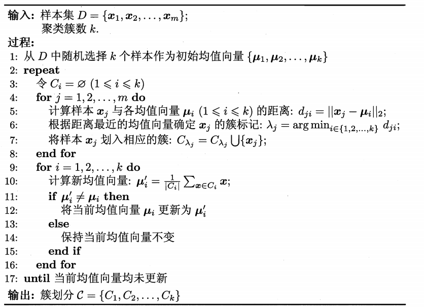

To prove that k-means converges, a sufficient condition is that the loss function is monotonic and bounded.

Monotonicity

The algorithm consists of two steps. The first assigns each point \(x\) to its nearest cluster, and the second recomputes the mean vectors.
First, consider the first step
If the cluster assignment of \(x_i\) does not change, the loss function clearly does not increase.
If the cluster assignment of \(x_i\) changes, then without loss of generality, consider

$$ J'=J-||x_i-\mu_k||_2^2+||x_i-\mu_{k'}||_2^2 $$

Because

$$ ||x_i-\mu_k||_2 \geq ||x_i-\mu_{k'}||_2 $$

the loss function does not increase.

Next, consider the second step
Without loss of generality, consider the loss function of a single cluster:

$$ J_i=\sum_{x\in{C_i}}||x-\mu_i||_2^2 $$

Let

$$ \frac{\partial J_i}{\partial \mu_i}=0 $$

Then we obtain

$$ \mu_i= \frac{1}{|C_i|}\sum_{x\in{C_i}}x=\mu'_i $$

The updated mean vector lies at the minimum point of the function, so this update step in the algorithm cannot increase the loss function.

In summary, the loss function in k-means decreases monotonically.

Boundedness

It is obviously bounded.

Therefore, the convergence proof of k-means is complete.

k-means vs. GMM

Unlike k-means, which uses prototype vectors to characterize cluster structure, Gaussian mixture clustering uses a probabilistic model to express cluster prototypes[1]:

$$ p_{\theta^{t}}(C_k|x_i) = \frac{p_{\theta^{t}}(C_k)p_{\theta^{t}}(x_i|C_k)}{\sum_j p_{\theta^{t}}(C_j)p_{\theta^{t}}(x_i|C_j)} $$

From this perspective, k-means also assumes a probability distribution[2]:

$$ p(C_j|x_i) = 1 \quad \mathrm{if} \quad \lVert x_i - \mu_j \rVert^2_2 = \min_k \lVert x_i - \mu_k \rVert^2_2 \\p(C_j|x_i) = 0 \quad \mathrm{otherwise} $$

By modifying this probability distribution, we can design an algorithm between k-means and GMM, for example using softmax:

$$ p(C_j|x_i) = \frac{\exp(- \alpha\lVert x_i - \mu_j \rVert^2_2)}{\sum_k \exp(- \alpha\lVert x_i - \mu_k \rVert^2_2)} $$

The new loss function is

$$ J = \sum_i \sum_j p(C_j|x_i) \lVert x_i - \mu_j \rVert^2 $$

Take the partial derivative:

$$ \frac{\partial{J}}{\partial{\mu_j}} = -2 \sum_i p(C_j|x_i) (x_i - \mu_j) $$

Set the derivative to zero, and we get the update formula for the mean vector:

$$ \mu_j = \frac{\sum_i p(C_j|x_i) x_i}{\sum_i p(C_j|x_i) } $$

For the original k-means pseudocode in [1], one only needs to replace the distance calculation on lines 5 and 6 with posterior probabilities, and replace line 10 with the formula above.

Advantages

1. Less sensitive to outliers
2. A generalized form of k-means
3. Still relatively simple to implement

Disadvantages

1. More hyperparameters need to be tuned (α)
2. Sensitive to initialization

k-means vs. RPCL

The idea of competitive learning can be introduced into k-means to learn the number of clusters automatically.
Define

$$ vector_i=\frac{1}{|C_i|}\sum_{x\in{C_i}}x-\mu_i $$

Combining the idea of RPCL, the update rule for the mean vectors is modified as follows:

$$ \mu'_i=\mu_i+learnrate \cdot vector_i\\ \mu'_k=\mu_k-learnrate \cdot penalty \cdot vector_i$$

where

$$ ||\mu_i-\mu_k||^2=min_{j \ne i}||\mu_i-\mu_j||^2\\ learnrate=const.,penalty=const. $$

If no point changes its cluster assignment, the algorithm terminates automatically, exactly as in the original k-means algorithm. Only the original second step is modified. The nearest mean vectors will automatically separate from each other, achieving the effect of determining the number of clusters automatically.

def k_means_with_RPCL(dataSet, k, dist_func=distEclud, 
                        createCent=randCent, lr=1, penalty=0.5):
    m = shape(dataSet)[0]
    dist_to_mu = mat(zeros((m,2)))
    centroids = createCent(dataSet, k)
    # used to determine whether clustering has converged; false means converged
    clusterChanged = True   
    while clusterChanged:
        clusterChanged = False
        # assign each data point to the nearest centroid
        for i in range(m):  
            minDist = inf  # minimum
            minIndex = -1
            for j in range(k):
                # compute the distance from data point i to centroid k
                distJI = dist_func(centroids[j, :], dataSet[i, :])  
                if distJI < minDist:
                    minDist = distJI
                    # if point i is closer to centroid j, assign i to j
                    minIndex = j 
            if dist_to_mu[i, 0] != minIndex : clusterChanged = True
            # store the assignment of data point i
            dist_to_mu[i, :] = minIndex, minDist**2  

        for cent in range(k):   # recompute the centroids
            secDist = inf  # second smallest
            secIndex = -1
            for i in range(k):
                if i != cent:
                    dist = dist_func(centroids[cent, :], centroids[i, :])
                    if dist < secDist:
                        secDist = dist
                        secIndex = i


            ptsInClust = dataSet[nonzero(dist_to_mu[:, 0] == cent)[0]]
            
            vector=(mean(ptsInClust, axis=0) - centroids[cent, :])
            centroids[cent, :] = centroids[cent, :] + lr * vector
            centroids[secIndex, :] = centroids[secIndex, :] - lr * penalty * vector

Clustering results
Set k=5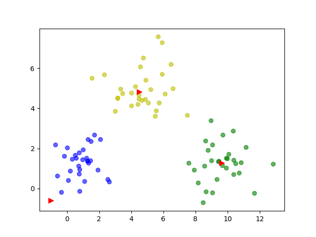

Set k=6

The expected effect is achieved.

References
[1.] Zhou Zhihua. Machine Learning[J]. 2016
[2.] EM Algorithm, K-means, and GMM Clustering https://sighsmile.github.io/2019-11-22-EM-KMeans-GMM/