Learning to Rank in Brief: From RankNet to LambdaMART

Chinese

This article gives a concise introduction to the background, taxonomy, and evaluation metrics of learning to rank, then reviews several classic algorithms from its development history. The goal is not to cover every technical detail, but to build an intuitive understanding of the core concepts behind ranking, as preparation for practical LTR applications in different scenarios.

Introduction

Background

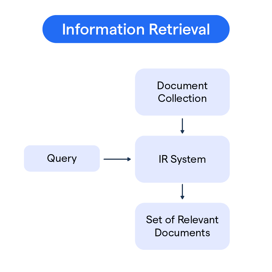
Learning to Rank (LTR) is a core technology in information retrieval. Search engines are the classic example: LTR is used to improve the final quality of ranked results, and it has been battle-tested for years. In each retrieval request, the user’s intent is called the query, and the candidate results are called documents. The search engine’s goal is to place the most relevant and highest-quality result first, the next best second, and so on. For a given query, an IR system first retrieves documents from a large database, often containing billions of pages. Because of performance constraints, retrieval is usually done in multiple layers and many parallel branches. The bottom layers may use simple keyword matching, while higher layers use more complex models. By the end, the candidate set is reduced to only a few dozen or a few hundred documents. Those candidates must then be ranked before being shown to the user. In this setting, the learning objective differs fundamentally from regression or ordinary classification:

1. The absolute relevance estimate of a document is not the point. Only relative order matters.
2. Most predictions do not matter because very few users browse deep into result pages. Only the top of the ranked list matters.

That is why learning to rank is needed.

Categories

LTR methods can usually be divided into three types: point-wise, pair-wise, and list-wise.

Point-wise LTR predicts the relevance of each document independently based on its own features, typically using mean squared error or cross-entropy loss, without modeling inter-document relationships. It is better viewed as a pseudo-LTR approach. Its advantage is simplicity and easy evaluation, so I will not discuss it further here.

Pair-wise LTR aims to predict the partial order between pairs of documents. As long as every pairwise relationship is predicted correctly, the ranked list will also be correct. That turns the problem into binary classification, commonly trained with cross-entropy loss. Compared with point-wise methods, pair-wise methods abandon absolute-score estimation and are better suited to ranking problems. RankNet is the representative example.

List-wise LTR treats the entire ranked list as one object and directly optimizes a list-level objective such as normalized discounted cumulative gain (NDCG). This is the most complete form of LTR: it avoids the difficulty of absolute-score estimation and prevents tail documents from dominating the learning signal. LambdaMART and ListNet are typical list-wise methods.

Evaluation Metrics

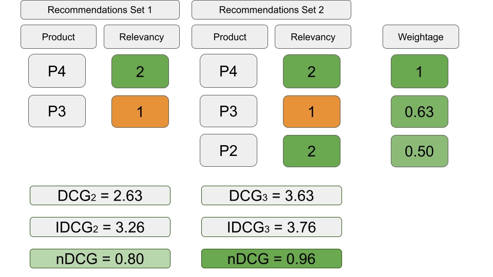
Normalized Discounted Cumulative Gain (NDCG) is one of the most widely used metrics in learning to rank, especially in information retrieval and search. It evaluates ranking quality while taking graded relevance into account.

1. Cumulative Gain (CG): for a ranked list of documents, CG is the sum of relevance scores up to position k:

$$ \text{CG@k} = \sum_{i=1}^{k} rel(i) $$

where \(rel(i)\) is the relevance score of the document at position \(i\), and \(k\) is the cutoff position.

2. Discounted Cumulative Gain (DCG): DCG applies a discount factor to relevance scores, reflecting the fact that lower-ranked documents usually contribute less to user satisfaction:

$$ \text{DCG@k} = \sum_{i=1}^{k} \frac{rel(i)}{\log_2(i+1)} $$

The denominator \(\log_2(i+1)\) decreases the contribution of documents as \(i\) increases.

3. Ideal DCG (IDCG): IDCG is the DCG of the ideal ranking, that is, the ranking sorted by true relevance. It serves as the normalization factor:

$$ \text{IDCG@k} = \sum_{i=1}^{k} \frac{rel_{\text{ideal}}(i)}{\log_2(i+1)} $$

4. Normalized DCG (NDCG): NDCG is the ratio between DCG and IDCG, normalized to the interval [0, 1], where 1 means a perfect ranking:

$$ \text{NDCG@k} = \frac{\text{DCG@k}}{\text{IDCG@k}} $$

The following figure shows a simple example of NDCG calculation.

Classic Algorithms

RankNet

Foundations

Structurally, RankNet is just a standard multilayer neural network for binary classification. What makes it special is the way it is trained and the objective it optimizes. Its key innovation is that cross-entropy loss, which does not look like a natural ranking loss, can nevertheless be used to solve ranking through gradient descent.

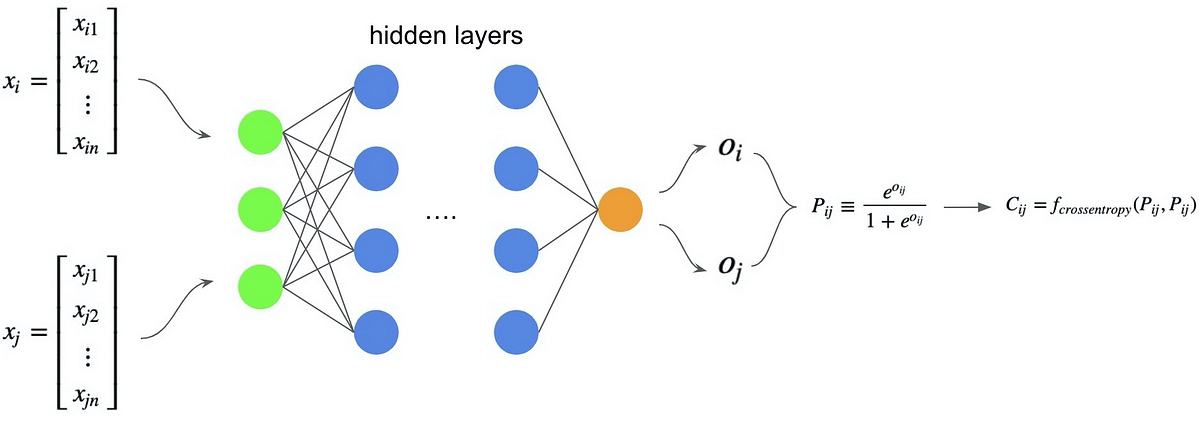
RankNet outputs a score \(s\) for document \(x\) and uses that score directly for ranking at inference time:

$$ s = f(x; w) $$

During training, the scores are converted into the probability that document \(x_i\) should be ranked ahead of \(x_j\), where \(\sigma\) is a hyperparameter:

$$ P_{ij} = P(x_i \triangleright x_j) = \frac{1}{1 + \exp(-\sigma \cdot (s_i - s_j))} $$

The cross-entropy loss is then defined as

$$ C_{ij} = -\hat{P}_{ij} \log P_{ij} - (1 - \hat{P}_{ij}) \log(1 - P_{ij}) = \frac{1}{2} (1 - S_{ij}) \sigma \cdot (s_i - s_j) + \log \left\{1 + \exp(-\sigma \cdot (s_i - s_j))\right\} $$

where \(S_{ij} \in {-1,0,+1}\) encodes the true pairwise relation.

The network can then be trained by gradient descent:

$$ w_k \rightarrow w_k - \eta \frac{\partial C_{ij}}{\partial w_k} $$

Improvement

The original RankNet has a practical problem: one query produces \(O(n^2)\) pairs, which is computationally expensive. A useful refinement is to treat all pairs from one query as a minibatch and perform a single gradient update. This is not merely an engineering trick; it is also the conceptual bridge toward later list-wise algorithms.

For one query, let the training set be \(I\), the set of document pairs with different labels, each pair included once and satisfying \(\forall (i,j) \in I, S_{ij}=1\). The accumulated gradient is

$$ \frac{\partial C}{\partial w_{k}} =\sum_{i} \lambda_{i} \frac{\partial s_{i}}{\partial w_{k}} $$

where

$$ \lambda_{i} \coloneqq \sum_{j:(i, j) \in I} \lambda_{i j}-\sum_{k:(k, i) \in I} \lambda_{k i} $$

and

$$ \lambda_{i j} \coloneqq \frac{\partial C_{i j}}{\partial s_{i}} $$

The key simplification comes from the symmetry of \(\lambda_{ij}\):

$$ \lambda_{i j} =\frac{\partial C_{i j}}{\partial s_{i}} =\sigma\left(\frac{1}{2}\left(1-S_{i j}\right)-\frac{1}{1+e^{\sigma\left(s_{i}-s_{j}\right)}}\right) = -\frac{\partial C_{i j}}{\partial s_{j}} $$

together with factorization:

$$ \begin{aligned} \frac{\partial C}{\partial w_{k}} &= \sum_{(i, j) \in I} \frac{\partial C_{i j}}{\partial w_{k}} \\ &= \sum_{(i, j) \in I}\left(\frac{\partial C_{i j}}{\partial s_{i}} \frac{\partial s_{i}}{\partial w_{k}}+\frac{\partial C_{i j}}{\partial s_{j}} \frac{\partial s_{j}}{\partial w_{k}}\right) \\ &=\sum_{(i, j) \in I} \lambda_{i j}\left(\frac{\partial s_{i}}{\partial w_{k}}-\frac{\partial s_{j}}{\partial w_{k}}\right) \\ &=\sum_{i} \left(\sum_{j:(i, j) \in I} \lambda_{i j}-\sum_{k:(k, i) \in I} \lambda_{k i}\right) \frac{\partial s_{i}}{\partial w_{k}} \\ &=\sum_{i} \lambda_{i} \frac{\partial s_{i}}{\partial w_{k}} \\ \end{aligned} $$

After simplification, each term corresponds to one candidate document. The term \(\frac{\partial s_{i}}{\partial w_{k}}\) depends only on model structure and parameters, while the \(\lambda\) value for a given URL \(U_1\) aggregates contributions from all other URLs with different labels under the same query. These \(\lambda\) values can also be interpreted as forces in a conservative field: if \(U_2\) is more relevant than \(U_1\), then \(U_1\) experiences a downward force of magnitude \(|\lambda|\) while \(U_2\) receives an equal upward force; if \(U_2\) is less relevant than \(U_1\), then the force directions reverse.

LambdaRank

RankNet solves the problem of relative order, but it still does not emphasize the top of the ranked list. It addresses only the first ranking requirement above, not the second. Consider the figure below: light gray bars are irrelevant URLs and dark blue bars are relevant URLs. On the left, the number of pairwise mistakes is 13. On the right, by moving a high-ranked URL down three slots and a relevant low-ranked URL up five slots, the pairwise mistake count decreases to 11. The total number of mistakes improves, but an IR metric such as NDCG, which emphasizes the top of the list, actually gets worse. The black arrows on the left show RankNet gradients, while the red arrows on the right show the direction we really want.

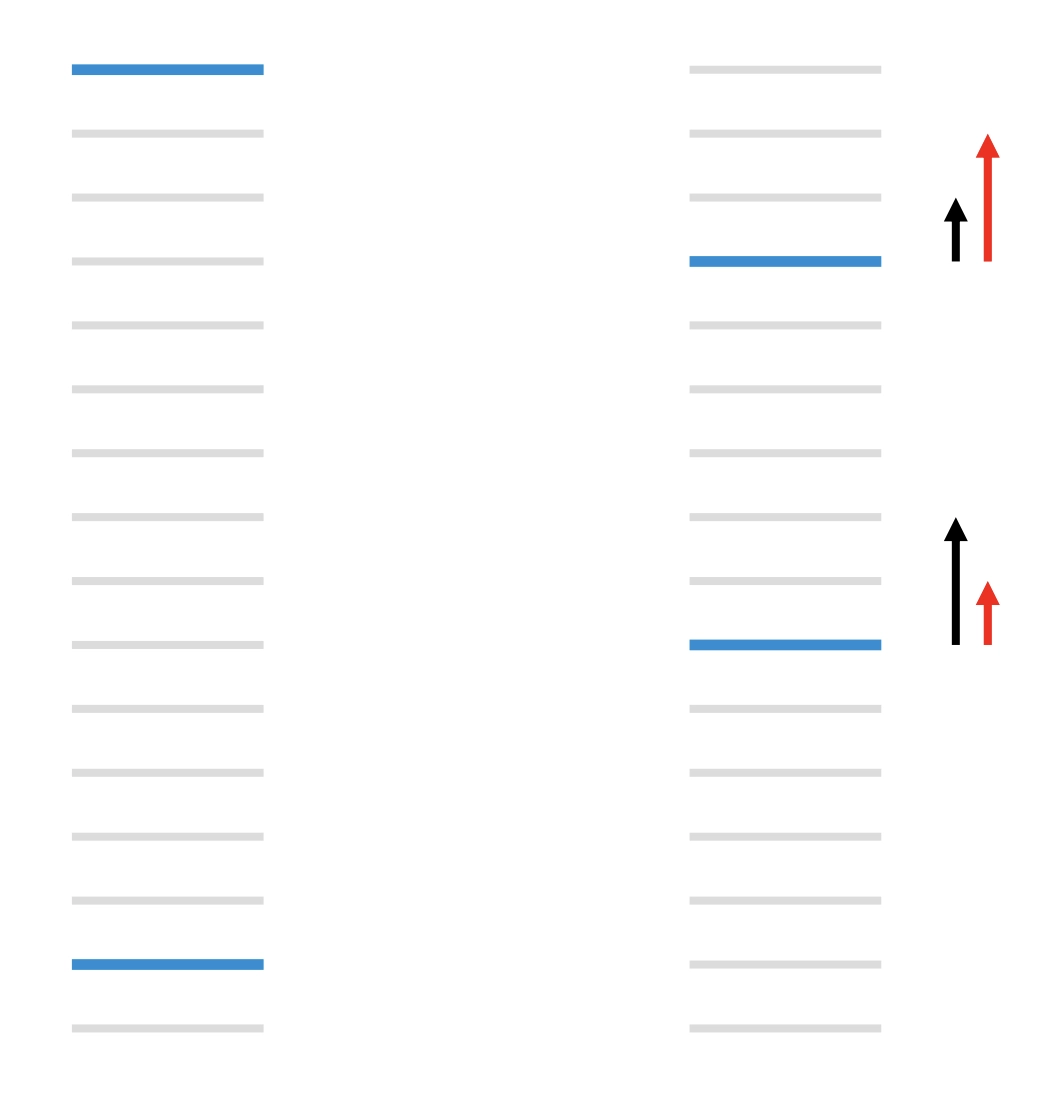
What we really want is a model that directly optimizes NDCG. To train that model, we do not need the loss itself; designing a good ranking loss is hard. We only need its gradient. Those arrow terms, the \(\lambda\) values, are exactly the gradients we need.

Experiments show that multiplying \(\lambda\) by the magnitude of the NDCG change induced by swapping two URLs, \(|\Delta_{NDCG}|\), gives very strong results. In LambdaRank we can imagine a utility \(C\) such that

$$ \lambda_{ij} = \frac{\partial C(s_i - s_j)}{\partial s_i} = \frac{-\sigma}{1+e^{\sigma(s_i-s_j)}} |\Delta_{NDCG}| $$

Since the goal is to maximize \(C\), the parameter update becomes

$$ w_k \rightarrow w_k + \eta \frac{\partial C}{\partial w_k} $$

which implies

$$ \delta C = \frac{\partial C}{\partial w_k} \delta w_k = \eta \left(\frac{\partial C}{\partial w_k}\right)^2 > 0 $$

So although IR metrics as functions of model scores are flat or discontinuous almost everywhere, LambdaRank bypasses the problem by working directly with gradients over sorted URLs. The method was validated empirically despite its initially weak theoretical foundation. If we want to optimize another ranking metric such as MRR or MAP, the only change is to replace \(|\Delta_{NDCG}|\) with the corresponding change in that metric.

LambdaMART

Basic Principle

Gradient-boosted decision trees are known by several names:

• MART - Multiple Additive Regression Trees
• GBDT - Gradient Boosting Decision Tree
• GBRT - Gradient Boosting Regression Tree

The goal of MART is to find a function \(f(x)\) such that

$$ \hat f(x) = \text{arg min}_{f(x)} E\Bigl[L\bigl(y, f(x)\bigr) \big| x\Bigr] $$

At the same time, MART is an additive model:

$$ \hat f(x) = \hat f_M(x) = \sum_{m = 1}^M f_m(x) $$

Training proceeds by adding new trees sequentially. Suppose \(m\) trees have already been fit. The target of iteration \(m+1\) is

$$ \delta \hat{f}_{m+1} = \hat{f}_{m+1} - \hat{f}_m = f_{m+1} $$

The update should reduce the loss:

$$ \delta L_{m+1} = L((x, y), \hat{f}_{m+1}) - L((x, y), \hat{f}_m) < 0 $$

Considering

$$ \delta L_{m+1} \approx \frac{\partial L((x, y), \hat{f}_m)}{\partial \hat{f}_m} \cdot \delta \hat{f}_{m+1}, $$

if we choose

$$ \delta \hat{f}_{m+1} = -g_{m} = -\frac{\partial L((x, y), \hat{f}_m)}{\partial \hat{f}_m}, \tag{2} $$

then necessarily \(\delta L_{m+1} < 0\). In short, MART reduces the loss by fitting the negative gradient.

MART needs a gradient, and LambdaRank defines exactly such a gradient. The two fit together naturally. Hence Lambda + MART = LambdaMART. LambdaMART has several major advantages:

• It bypasses the need to define a ranking loss explicitly and instead uses gradients to optimize ranking metrics such as NDCG directly, which are list-level metrics aligned with user experience.
• Its model structure is GBDT, so it inherits the strengths of decision trees: resistance to overfitting, robustness to outliers, and fast training.

LambdaMART Algorithm Flow

1. Set parameters

   • Number of trees: \(N\)
   • Number of training samples: \(m\)
   • Number of leaves per tree: \(L\)
   • Learning rate: \(\eta\)

2. Initialization
   For \(i = 0\) to \(m\):

   • \(F_0(x_i) = \text{BaseModel}(x_i)\)

3. Tree-building loop

• For \(k = 1\) to \(N\):

  • For \(i = 0\) to \(m\):
    • \(y_i = \lambda_i\)
    • \(w_i = \frac{\partial y_i}{\partial F_{k-1}(x_i)}\)
  • End for
  • Partition the data into \(L\) leaves: \({R_{lk}}_{l=1}^L\)
  • Compute leaf values:
    • \(\gamma_{lk} = \frac{\sum_{x_i \in R_{lk}} y_i}{\sum_{x_i \in R_{lk}} w_i}\)
  • Update the model:
    • \(F_k(x_i) = F_{k-1}(x_i) + \eta \sum_{l} \gamma_{lk} I(x_i \in R_{lk})\)

• End for

PS: for more detail, I recommend the original reading material.