From Chatterjee's Correlation to Tau-Star: Completeness and Power in Independence Testing

Chinese

In the earlier article Three Measures for Sequence Correlation, I introduced Chatterjee’s correlation coefficient, which can detect nonlinear and non-monotonic associations between variables. Its form is simple, computation is fast, and it is especially suitable for screening input features for nonlinear machine learning models. New research, however, shows that its detection efficiency is inadequate for some non-functional dependence structures. This article first reviews and expands on the concrete mechanics and key properties of Chatterjee’s \(\xi\). It then introduces an alternative: the equally consistent, distribution-free independence test statistic \(\tau^*\).

A Review of Chatterjee’s Correlation

Definition

When discussing correlation, we use the term correlation measure for a population parameter and correlation coefficient for a sample statistic, denoted with the subscript \(n\). Let \(F\) denote the joint bivariate distribution of the random pair \((X^{(1)}, X^{(2)})\), and let \(F_1\) and \(F_2\) denote the corresponding marginal distributions.

Let \((X_{[1]}^{(1)}, X_{[1]}^{(2)}), \dots, (X_{[n]}^{(1)}, X_{[n]}^{(2)})\) be a reordering of the sample such that \(X_{[1]}^{(1)} \le \dots \le X_{[n]}^{(1)}\). If \(F_2\) is continuous, and if we additionally assume \(X_1^{(2)}, \dots, X_n^{(2)}\) are all distinct, then \(r_{[i]}\) denotes the rank of \(X_{[i]}^{(2)}\) among \(X_{[1]}^{(2)}, \dots, X_{[n]}^{(2)}\). In practice, ties have limited impact, so I do not focus on them here.

Definition. The Chatterjee correlation coefficient \(\xi_n\) is

$$\xi_n = 1 - \frac{3 \sum_{i=1}^{n-1} |r_{[i+1]} - r_{[i]}|}{n^2 - 1}.$$

Intuitively, Chatterjee’s correlation measures whether neighboring values of \(X^{(2)}\) remain close after sorting by \(X^{(1)}\).

Chatterjee (2021) proved that \(\xi_n\) estimates the Dette-Siburg-Stoimenov rank correlation measure

$$\xi = \frac{\int \operatorname{Var}(E[I(X^{(2)} \ge x) \mid X^{(1)}]) dF_2(x)}{\int \operatorname{Var}(I(X^{(2)} \ge x)) dF_2(x)}.$$

This expression looks very much like the coefficient of determination \(R^2\), namely \(\frac{\text{Explained Variance}}{\text{Total Variance}}\). In fact, that is essentially what it is, but defined in a broader and more general nonparametric framework: the task of “using \(X^{(1)}\) to predict \(X^{(2)}\)” is decomposed into binary classification problems over all thresholds \(x\), and the explained-variance ratio for each binary problem is then averaged.

Fix a threshold on \(X^{(2)}\) and define the binary label \(Y_x=\mathbf{1}{X^{(2)}\ge x}\). Then \(E[Y_x\mid X^{(1)}]\) is the conditional probability that \(X^{(2)}\) exceeds the threshold \(x\) given \(X^{(1)}\).

For any random variable, total variance can be decomposed as

$$ \operatorname{Var}(Y_x)=\underbrace{E\big[\operatorname{Var}(Y_x\mid X^{(1)})\big]}_{\text{irreducible noise}} +\underbrace{\operatorname{Var}\big(E[Y_x\mid X^{(1)}]\big)}_{\text{explained by }X^{(1)}} $$

\(\operatorname{Var}(E[Y_x\mid X^{(1)}])\) measures how much this conditional probability fluctuates across different values of \(X^{(1)}\). The larger the fluctuation, the more \(X^{(1)}\) is truly changing the probability of crossing the threshold, and the stronger its predictive power.

The denominator \(\operatorname{Var}(Y_x)=p_x(1-p_x)\) is the baseline uncertainty of that binary task itself. Finally, \(\xi\) integrates over all thresholds \(x\) using \(F_1\) and \(F_2\) as weights, which amounts to averaging over all quantiles.

$$ \xi = \frac{\displaystyle \int \underbrace{\operatorname{Var}\big(E[\mathbf{1}\{X^{(2)}\ge x\}\mid X^{(1)}]\big)}_{\text{the part explained by }X^{(1)}\text{ (cross-}X^{(1)}\text{ variation)}} dF_2(x)} {\displaystyle \int \underbrace{\operatorname{Var}\big(\mathbf{1}\{X^{(2)}\ge x\}\big)}_{\text{total variance (baseline uncertainty at threshold }x\text{)}} dF_2(x)} $$

Properties

This measure \(\xi\) and its sample estimator \(\xi_n\) have attracted strong interest in modern statistics because they possess several striking properties:

Key Property 1: Capturing Nonlinear and Non-Monotonic Relations

The traditional Pearson \(\rho\) captures only linear relationships. Spearman \(\rho\) and Kendall \(\tau\) capture only monotonic relationships. The advantage of \(\xi\) is that it can detect any functional relationship, including non-monotonic relationships such as a U-shaped dependence \(Y = X^2\), or even more complex structures. For example, if \(Y = X^2\) with \(X \sim U(-1, 1)\), both Pearson and Spearman correlations are close to 0, while \(\xi\) converges to a positive value and correctly indicates that \(Y\) depends entirely on \(X\).

Key Property 2: Asymmetry

Pearson, Spearman, and Kendall are all symmetric: \(\rho(X, Y) = \rho(Y, X)\).

\(\xi\) is asymmetric.

• \(\xi(X^{(1)}, X^{(2)})\) measures the degree of dependence from \(X^{(1)}\) to \(X^{(2)}\).
• \(\xi(X^{(2)}, X^{(1)})\) measures the degree of dependence from \(X^{(2)}\) to \(X^{(1)}\).

These two values are usually not equal. \(\xi\) therefore allows us to quantify one-directional predictive strength in a way that resembles causal asymmetry.

Key Property 3: Easy to Compute

The construction uses the indicator function \(\mathbf{1}{X^{(2)}\ge x}\) and integrals over the distribution function \(F\), making it insensitive to arbitrary monotone transformations and naturally robust. It is model-free and fully nonparametric.

Once the sample is sorted by \(X^{(1)}\), a single sequential scan can accumulate the “jump size” of neighboring \(X^{(2)}\) values. In implementation, the complexity can reach \(\mathbb{O}(n\log n)\), and in NumPy it only takes a few lines.

Theoretical Elegance, Practical Power Limitations

The reason Chatterjee’s coefficient \(\xi_n\) caused such excitement in 2021 is that the population quantity \(\xi\) has a remarkable theoretical property: \(\xi=0\) if and only if the two variables \(X^{(1)}\) and \(X^{(2)}\) are independent. In theory, this makes it a “complete” measure of independence, superior to traditional coefficients that capture only linear dependence (Pearson \(\rho\)) or monotonic dependence (Spearman \(\rho\)).

However, Shi et al. (2021) pointed out that although the theoretical definition of \(\xi\) is elegant, the independence test based on its sample statistic \(\xi_n\) suffers from severe power deficiencies. In other words, \(\xi_n\) is consistent but inefficient as a test for independence, and under some local alternatives it is nearly useless.

This weakness can be understood on two levels.

Weak Numerical Signal in Finite Samples

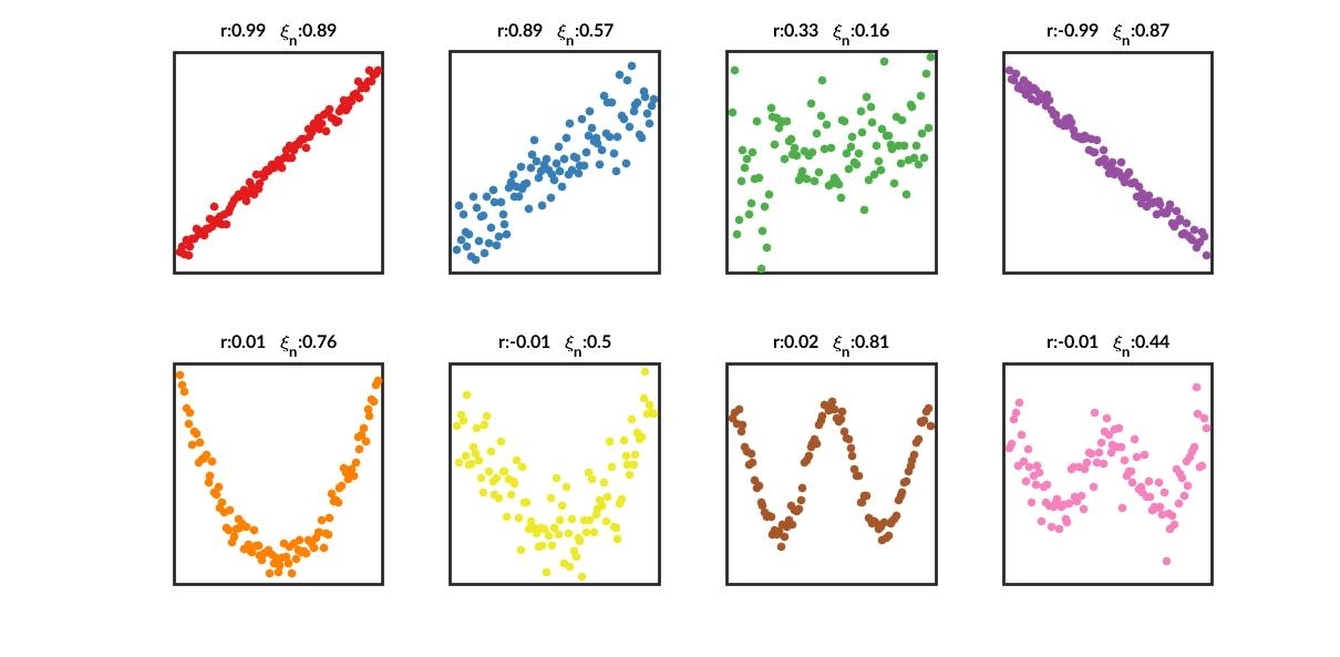
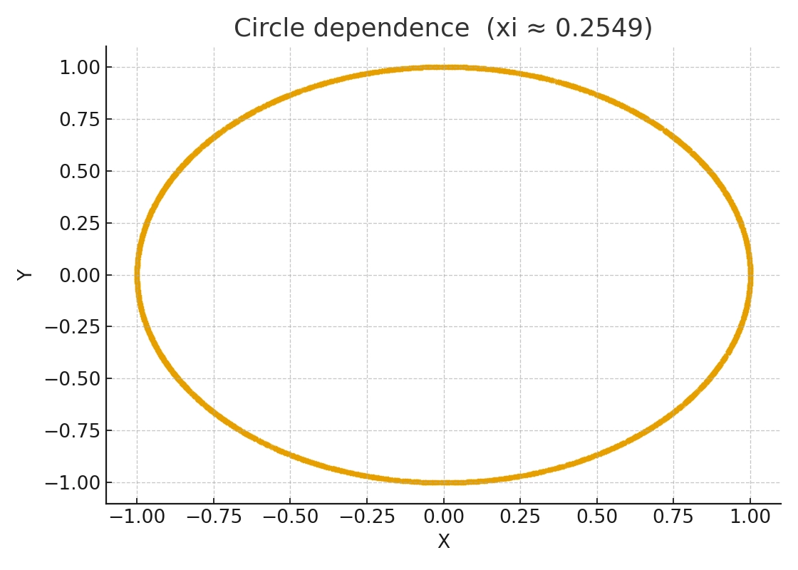
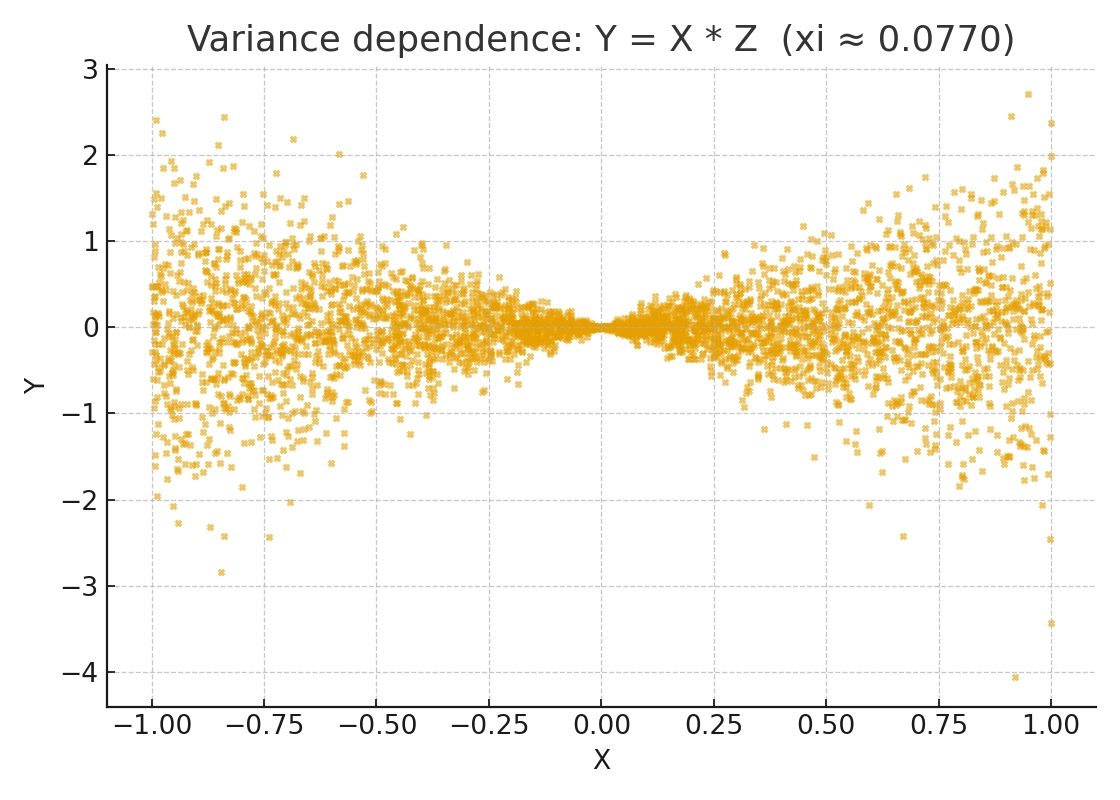
At its core, \(\xi\) measures the variation in the conditional expectation \(E[I(X^{(2)} \ge x) \mid X^{(1)}]\) as \(X^{(1)}\) changes. For some specific dependence structures, such as symmetric non-monotonic patterns like U-shapes or circles, or purely heteroskedastic dependence, this variation may itself be very small or even largely cancel out.

As a result, for these “shape dependence” structures, the theoretical value of \(\xi\) is indeed positive, but it may be numerically tiny. In finite samples, such a weak signal in \(\xi_n\) is easily drowned out by noise, making the observed value look close to 0. The issue is not that \(\xi\) is theoretically 0, but that the signal is weak and the convergence of \(\xi_n\) toward that small truth is slow.

Low Asymptotic Power

This insensitivity to certain shapes directly leads to the statistic’s fatal weakness in hypothesis testing. The paper proves this through a local-power analysis.

Suppose the alternative hypothesis is very weak, with dependence shrinking at the rate \(n^{-1/2}\) as the sample size increases. Under such a local alternative, the power of the \(\xi_n\) test collapses completely. The paper’s Theorem 1 shows that in this setting, the power of the \(\xi_n\) test converges to \(\alpha\), the nominal significance level, such as 5%.

That means the \(\xi_n\) test becomes no better than blind guessing when signals are weak: it cannot distinguish weak but real dependence from pure random noise.

By contrast, classical coefficients such as Hoeffding’s \(D\), Blum-Kiefer-Rosenblatt’s \(R\), and Bergsma-Dassios’s \(\tau^*\) remain rate-optimal under the same weak signals. They retain nontrivial power and remain sensitive to this kind of dependence.

Not a Universal Detector of Independence

Shi et al. (2021) proved that \(\xi_n\) is rate sub-optimal. Its theoretical form is elegant and its computation is efficient at \(O(n \log n)\), but if the core goal is testing independence, it is not sensitive enough. In practice, when we observe a very small \(\xi_n\), we cannot conclude that the variables are truly independent; there may still be a non-functional or weak dependence that \(\xi_n\) simply fails to detect effectively.

Any feature that is not independent theoretically contains predictive information and is therefore statistically “valuable.” From a machine-learning perspective, non-independence implies potential predictability. In quantitative investing, the weakness of \(\xi_n\) often means mistakenly discarding a feature that has predictive power for risk.

Tau-Star: Another Rank-Based Independence Test

\(\tau^*\) (tau-star) is a consistent independence-testing statistic proposed by Bergsma & Dassios (2014). It is a generalized version of Kendall’s \(\tau\). In practice, it is more suitable for serious independence testing, whereas \(\xi_n\) is better suited to fast nonlinear feature screening.

Kendall’s \(\tau\) is defined as

$$ \tau = E[\operatorname{sign}(X_1 - X_2)\operatorname{sign}(Y_1 - Y_2)] $$

It reflects the difference between the probabilities of concordant and discordant pairs. But \(\tau\) may equal 0 under some non-monotonic dependence structures even when \(X\) and \(Y\) are not independent, so it is not consistent for independence testing.

Definition:

Building on this, Bergsma and Dassios defined a new dependence measure:

$$ \tau^* = E[a(X_1, X_2, X_3, X_4)a(Y_1, Y_2, Y_3, Y_4)] $$

where \(a\) is a quadruple-based “sign covariance” function.

$$ a(z_1, z_2, z_3, z_4) = \operatorname{sign}\left(|z_1 - z_2| + |z_3 - z_4| - |z_1 - z_3| - |z_2 - z_4|\right) $$

The sample statistic is

$$ t^* = \frac{1}{\binom{n}{4}} \sum a(x_i,x_j,x_k,x_l)\,a(y_i,y_j,y_k,y_l) $$

In the continuous case without ties, this measure satisfies

$$ \tau^* \ge 0 \quad \text{and} \quad \tau^* = 0 \iff X, Y \text{ are independent} $$

Thus it yields a consistent independence test.

\(\tau\) concerns whether two points move in the same direction;
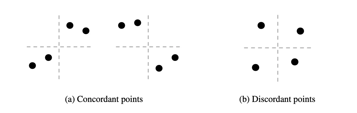
\(\tau^*\) instead examines the joint relative ordering of four points.

Define a quadruple \(({(x_1,y_1),…,(x_4,y_4)})\):

• If one coordinate axis can split the four points so that the two pairs are ordered consistently in both \(X\) and \(Y\), or reversed in both, then the quadruple is called concordant.
• If one pair is concordant and the other is discordant, then the quadruple is called discordant.

Bergsma & Dassios proved that

$$ \tau^* = \frac{2P(\text{concordant quadruples}) - P(\text{discordant quadruples})}{3} $$

and under independence, the probability of concordant quadruples equals \(1/3\) while the probability of discordant quadruples equals \(2/3\). Once \(X\) and \(Y\) follow any systematic pattern, whether linear, curved, periodic, or ring-shaped, the distribution of relative orderings departs from the independent case, increasing the probability of concordant quadruples and producing \(\tau^* > 0\).

In practice, independence testing with \(\tau^*\) is implemented through a permutation test.

If one wants to use \(\tau^*\) as a dependence measure scaled between 0 and 1, a normalized version can be used:

$$ \tau_b^* = \frac{\tau^*(X, Y)}{\sqrt{\tau^*(X, X) \tau^*(Y, Y)}} $$

\(\tau_b^* \in [0,1]\), with 1 corresponding to a noiseless functional relationship.

Summary

Chatterjee’s coefficient \(\xi_n\) breaks the task of “using \(X\) to predict \(Y\)” into binary classification problems across all thresholds and characterizes predictive power through

$$ \operatorname{Var}\big(P(Y\ge x\mid X)\big) $$

The corresponding population quantity \(\xi\) satisfies \(\xi=0 \iff X\perp Y\), and for functional dependence, including non-monotonic functions, \(\xi=1\). In terms of expressiveness, it is “complete.” At the same time, \(\xi_n\) can be computed in \(O(n\log n)\) time and is therefore very well suited as a fast scoring statistic for nonlinear, non-monotonic correlation in large-sample feature screening.

The problem is that Shi, Drton, and Han showed that under certain symmetric or variance-driven local alternatives, the true value of \(\xi\) itself is extremely close to 0, and \(\xi_n\) is almost insensitive to weak dependence at the \(n^{-1/2}\) scale. Its asymptotic power degrades to the significance level \(\alpha\), making it rate sub-optimal. So although \(\xi_n\) is a consistent independence-test statistic, it is not a high-power universal detector of independence.

Bergsma-Dassios’s \(\tau^*\) instead uses the relative ordering of quadruples as rank information. In the continuous case it satisfies

$$ \tau^* \ge 0,\quad \tau^* = 0 \iff X\perp Y, $$

providing a consistent test for arbitrary dependence and achieving rate-optimal local power, at the cost of greater computational complexity.

Accordingly, a sensible division of labor in practice is:

• \(\xi\) for fast screening of nonlinear features
• \(\tau^*\) for serious testing of whether variables are independent, especially in risk modeling

Comparison of Correlation Statistics

Metric	Linear / Monotonic	Arbitrary Dependence	Distribution-Free	Local Power \((n^{-1/2})\)	Computation
Pearson \(\rho\)	Linear	No	No	Suboptimal	Extremely fast
Spearman / Kendall	Monotonic	No	Partial	Suboptimal	Fast
\(\xi\)	Functional, including non-monotonic	In principle yes	Yes	Suboptimal (symmetric / non-monotonic classes)	Fast \(O(n\log n)\)
\(\tau^{*}\)	Arbitrary	Yes	Yes	Optimal	\(O(n\log n)\) after optimization

---

References

• Bergsma, Wicher, and Angelos Dassios. 2014. “A Consistent Test of Independence Based on a Sign Covariance Related to Kendall’s Tau.” Bernoulli 20 (2). https://doi.org/10.3150/13-BEJ514.
• Chatterjee, Sourav. 2021. “A New Coefficient of Correlation.” Journal of the American Statistical Association 116 (536): 2009–22. https://doi.org/10.1080/01621459.2020.1758115.
• Shi, H, M Drton, and F Han. 2022. “On the Power of Chatterjee’s Rank Correlation.” Biometrika 109 (2): 317–33. https://doi.org/10.1093/biomet/asab028.