A Simple Introduction to Backtest Overfitting
In quantitative trading, few problems are more frustrating than a strategy going live and then performing far worse than expected. The goal of this article is to give readers a first-pass understanding of what “backtest overfitting” means, why it happens, and what can be done about it.
Problem Definition
What is a backtest
If you design a strategy purely from deduction, such as arbitraging explicit trading rules, then you do not need a backtest. But if you want to design a strategy by inducing patterns from historical markets, you need to simulate trading in historical environments and evaluate performance. In this article, the discussion is narrowed further: researchers run backtests in order to select the best strategy from a pool of candidate strategies.
For example, I design a momentum strategy: “hold the stock in the universe with the largest gain over the past W days using the full position.” But I want to know how to choose W. A typical backtest is to set W = 5, 10, and 15, then simulate trading on data from 2012 to 2022. Here the Sharpe ratio is used as the performance metric.
| Strategy ID | W | \(SR_{IS}\) |
|---|---|---|
| 1 | 5 | 0.4 |
| 2 | 10 | 1.1 |
| 3 | 15 | 0.8 |
I observe that the Sharpe ratio is best when W = 10, so I deploy W = 10 in live trading. This process of evaluating models and choosing one is what this article calls a backtest.
What is backtest overfitting
In practice, backtests often fail: it is easy to tweak parameters until a model produces a very high Sharpe ratio on historical data, but very hard to make real money live.
In general, \(E[SR_{OOS}]<SR_{IS}\) (IS means in-sample, OOS means out-of-sample). The Sharpe ratio from a backtest often decays badly on future data for many reasons: market patterns change, model variance is too high, and so on. But here we only consider overfitting caused by strategy selection. In other words, even if expected future returns are not that good, or even if every strategy loses money, the backtest is still a success as long as \(S_2\) remains the best-performing strategy in the set. If the selected \(S_2\) ends up near the bottom in the future, then running the backtest actually made me lose more money. I would have been better off choosing a strategy at random.
| Strategy ID | W | \(SR_{IS}\) | \(SR_{OOS}\) | \(Rank_{IS}\) | \(Rank_{OOS}\) |
|---|---|---|---|---|---|
| 1 | 5 | 0.4 | ? | 1 | ? |
| 2 | 10 | 1.1 | ? | 3 | ? |
| 3 | 15 | 0.8 | ? | 2 | ? |
This leads to the definition of backtest overfitting: the best strategy selected from the candidate pool based on historical performance ends up in the bottom half of the ranking in the future.
$$ E[Rank_{OOS, selected}] < K/2 $$
Here K is the number of candidate strategies.
The probability of backtest overfitting (PBO) is
$$ P(Rank_{OOS, selected} < K/2 | Rank_{IS, selected} = K) $$
The biggest difference between backtest overfitting and overfitting in machine learning is that machine learning changes a model’s parameters, while backtesting only chooses among different models. Their common feature is that improving in-sample performance can lead to degraded out-of-sample performance.
Problem Analysis
Causes
Why does backtest overfitting occur? The selection rule above simply chooses the strategy with the highest historical Sharpe ratio, and that may also be the most widely used method. It contains an implicit assumption: that \(SR_{IS}\) and \(SR_{OOS}\) are at least positively correlated. In reality they may be unrelated or even negatively correlated. There are two reasons: multiple testing and environmental change.
First, as long as I run enough experiments, I can always find a strategy that looks good on historical data, whether train, validation, or test. A strategy selected this way is almost guaranteed to perform poorly in the future. This behavior is also called multiple testing or p-hacking. If the goal is simply to produce an attractive result, exploiting selection bias may be understandable. But deliberately doing so in practical backtesting is a bad idea.
Second, future financial data is not i.i.d. with historical data. In supervised learning, overfitting happens because a model learns the training set too hard and ends up with excessive variance. Strategy failure is closer to a reinforcement learning model that cannot perform well in a different environment: the generalization ability is weak. A strategy may fit the “true model” of that time very well, but the “true model” changes in the future.
The ideal backtesting system would separate the patterns a strategy relies on into two parts: those that will reappear in the future and those that will never appear again. Then it could measure generalization precisely. But that is obviously even harder than designing a consistently profitable strategy, so it is unrealistic. A more practical goal is for a backtest to choose a reasonably good model from the candidate pool, or at least avoid losing extra money because of model selection. Ideally it should also output PBO and an estimate of future performance decay.
Combining with machine learning algorithms
Because machine learning algorithms learn from historical data and train model parameters, the data used for training cannot also be used to evaluate the model. Backtesting evaluates the model output by the algorithm, so it occupies the role of the test set. If data from 2010 to 2018 is used for training, including both train and validation, then data after 2019 should be used for backtesting.
Several Approaches
Traditional methods
From a statistical point of view, if a strategy’s Sharpe ratio is high enough, the discovery is significant. But running more experiments makes it more likely to find a high Sharpe ratio by chance, so the standard has to be raised: a Sharpe ratio of 2 may be enough after one experiment, but after ten experiments you may demand 3 instead. In that case a strategy with Sharpe ratio 2 is treated as noise. Similar approaches include limiting the total number of trials or requiring a longer backtest period. These threshold-adjustment methods can solve, and can only solve, the part of backtest overfitting caused by multiple testing.
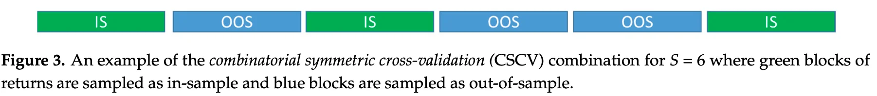
Combinatorially symmetric cross-validation
The idea of combinatorially symmetric cross-validation (CSCV) is to repeat the model selection process ten thousand times, estimate the frequency of backtest overfitting as the expected PBO, and also estimate the relationship between \(SR_{IS}\) and \(SR_{OOS}\). The concrete method is to split the dataset in many combinations and simulate the process of selecting a strategy based on in-sample performance.
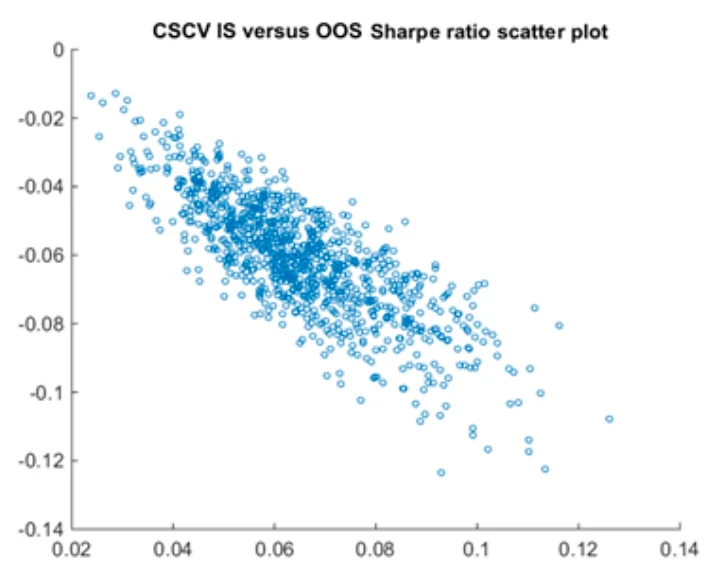
CSCV divides the return matrix \(R^{T \times K}\) into S blocks. One half is used as simulated IS data \(R^{T/2 \times K}\) and the other half as simulated OOS data \(R^{T/2 \times K}\) . There are \(C_S^{S/2}\) combinations, so the model selection process is repeated that many times. If, across all these selections, \(Rank_{IS}\) and \(Rank_{OOS}\) have little relationship, then the probability of backtest overfitting in this candidate set is high. The relationship between \(SR_{IS}\) and \(SR_{OOS}\) can also be summarized as an estimate of future decay for the selected strategy.
The downside of CSCV is that it can only produce one PBO for an entire candidate set; it cannot evaluate a single strategy. It also makes a visibly biased prediction of the relationship between \(SR_{IS}\) and \(SR_{OOS}\). Consider a set of strategies with the same average return. The best strategy selected in IS will almost certainly look worse in OOS. For \(Rank_{IS,best}\) and \(Rank_{OOS,best}\) to be close, one strategy must be consistently superior on the whole dataset. In my view, CSCV is essentially a new algorithm for adjusting the threshold.
Bayesian inference
The idea of Bayesian inference is to model the backtesting process with random variables and compute the posterior distributions of those variables from the backtest data. Once we have posterior distributions for these parameters, we can generate new data from the same distribution and compute any quantities we care about, such as PBO and haircut.
The most naive model assumes that each row of the return matrix follows a multivariate normal distribution.
$$ R_t=[r_{t,1},r_{t,2}...r_{t,K}] \sim N(\mu,\Sigma) $$
Use MCMC to estimate the distributions of \(\mu\) and \(\Sigma\), generate ten thousand new datasets, and simulate the model selection process ten thousand times. Then PBO, haircut, and similar metrics can be estimated.
To improve this model, introduce a latent variable \(\gamma \sim Ber(p)\) to indicate whether a strategy is a true discovery:
$$ R_t=[r_{t,1},r_{t,2}...r_{t,K}] \sim N(\mu^*,\Sigma)\\ \mu^*_i=\gamma_i \mu $$
A Simple Introduction to Backtest Overfitting