[AMM Quant Deep Dive 01] Understanding the Economic Essence of AMMs: From Impermanent Loss (IL) to Loss-Versus-Rebalancing (LVR)

Chinese

Many people treat providing liquidity (LP) on on-chain exchanges (DEXs) such as Uniswap as a passive form of “yield management” or “mining.” That is an extremely dangerous misunderstanding. From the perspective of market microstructure, an AMM is fundamentally an adverse-selection game arena defined by an algorithm.

This article is the first entry in the [AMM Quant Deep Dive] series. We will abandon the traditional retail-investor perspective, start from macro market equilibrium, strip away the disguise of “impermanent loss (IL)” through rigorous mathematical derivation, and introduce the true core risk metric for professional AMM market making: Loss-Versus-Rebalancing (LVR).

Introduction

With the rise of DeFi and on-chain automated market makers (AMMs), we are living through a paradigm shift in financial infrastructure. This is not merely a technical iteration. It is an irreversible historical trend.

Yet even in this wave, many professional quant practitioners still find themselves evaluating protocols like Uniswap through the mental model of centralized exchanges.

If we stop at the surface-level yield story of “deposit tokens and earn interest,” or if we still use a path-independent metric like impermanent loss (IL) to measure risk, then we are not only severely underestimating tail risk, but also missing the essential nature of this new market microstructure.

A Macro View: The Economics of AMMs

An Intuitive Interpretation

AMMs are easier to understand if we compare them with the more familiar limit order book (LOB) of traditional finance. In a traditional LOB market, market makers provide liquidity by posting asks above the current price and bids below it. These quotes are adjusted dynamically in real time.

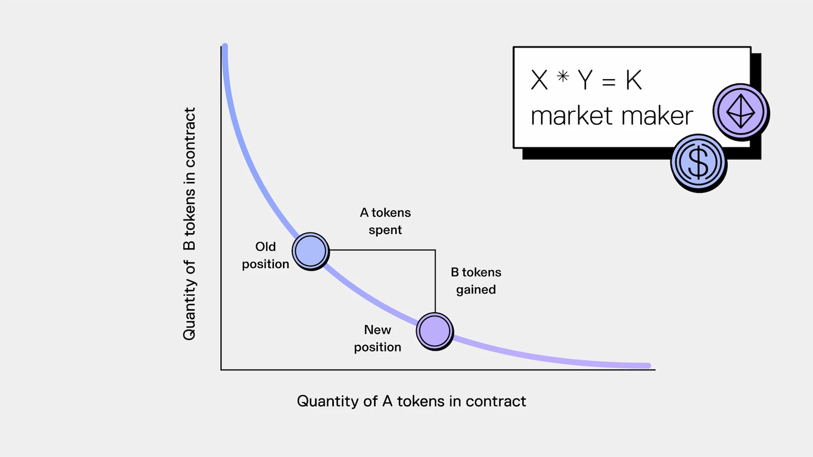
An AMM is essentially an order book maintained automatically by an algorithm. In AMMs, especially constant-product market makers, liquidity providers (LPs) are passive. In the classic Uniswap V2 model \(x \cdot y = k\), liquidity is spread uniformly over the price range \((0, \infty)\). That means the pool always has assets available for trade, whether the price rises to \(1000 or falls to \)0.01. Mathematically, this is equivalent to placing infinitely small buy and sell orders at every price level in an order book. In that setting, price discovery depends entirely on external arbitrageurs.

Endogenous Equilibrium

The core contribution of Lehar & Parlour is to treat AMM liquidity supply as an endogenous variable. Pool size is not random. It is the Nash equilibrium outcome of the game between LPs and arbitrageurs.

Scenario Setup

When the external market price jumps, the AMM quote lags behind. Arbitrageurs then execute a trade that pushes the AMM price back in line with the external market.

• LP revenue (\(\Pi_{LP}\)): trading fees generated by trades.
• LP cost (\(L_{arb}\)): losses caused by arbitrageurs entering after an external price jump, that is, adverse-selection cost.

Under free entry and exit, as long as expected profit \(\Pi_{LP} > 0\), new capital enters the pool; otherwise capital leaves. Therefore, in equilibrium, \(\Pi_{LP} = 0\) after accounting for opportunity cost.

The Key Mechanism: Price Impact as the Control Valve

In an AMM, price impact is deterministic and depends on pool depth (\(T_0\)).

• A larger pool (\(T_0 \uparrow\)) \(\rightarrow\) lower price impact.
• A smaller pool (\(T_0 \downarrow\)) \(\rightarrow\) higher price impact.

The Arbitrageur’s Profit-Maximization Problem

Assume the external price experiences a jump of size \(\sigma\). The arbitrageur must choose the trade size (\(t_{arb}\)) that maximizes profit.
The arbitrageur’s profit function \(\pi_{arb}\) is

$$ \pi_{arb} = \underbrace{(\text{new price} - \text{average execution price})}_{\text{spread capture}} \times t_{arb} $$

Since the average execution price depends on trade size \(t_{arb}\) and pool depth \(T_0\), a deeper pool means the average execution price stays closer to the old price, giving the arbitrageur more room to profit.

Conclusion A: The larger the pool depth \(T_0\), the larger the optimal arbitrage size \(t_{arb}^*\) required to eliminate the price gap.

$$ \frac{\partial t_{arb}^*}{\partial T_0} > 0 $$

The LP Loss Function

LP losses are directly equal to arbitrageur profits under a zero-sum assumption.

$$ L_{arb} \propto t_{arb}^* \times \sigma $$

Combining this with Conclusion A leads to an important and counterintuitive implication: the deeper the pool, the larger the total LP loss from a single price jump, because the arbitrageur can consume more liquidity at more favorable prices.

Equilibrium Derivation

The LP net-profit function is

$$\text{Net Profit} = \text{Fees}(T_0) - \underbrace{\text{Loss}(T_0, \sigma)}_{L_{arb} \propto t_{arb}^* \times \sigma}$$

• Effect of volatility \(\sigma\): When volatility \(\sigma\) rises, the loss term increases sharply. To preserve Net Profit = 0, \(T_0\) must shrink, increasing price impact and forcing arbitrageurs to reduce optimal trade size \(t_{arb}^*\), which lowers the loss term.

  $$ \sigma \uparrow \Rightarrow \text{Equilibrium } T_0 \downarrow $$

• Effect of noise trading: When noise-trading volume increases, the fee term rises. LP provision becomes profitable, capital flows in, and \(T_0\) rises until marginal profit returns to zero.

  $$ \text{Noise} \uparrow \Rightarrow \text{Equilibrium } T_0 \uparrow $$

Summary: The equilibrium pool size is a resistance mechanism spontaneously formed by LPs to defend themselves against arbitrageurs. Under high volatility, pools become shallow because LPs are raising slippage, that is, price impact, to drive arbitrageurs away. This explains why slippage tends to be large for highly volatile assets on Uniswap, where pools are shallow, but tiny for stablecoin pairs. In effect, LPs use fees from noise traders to subsidize arbitrageur profits.

Lehar & Parlour provide a closed-form equilibrium solution for token supply \(T_0\), quantifying the exact balance between “revenue” and “attack cost”:

$$ T_{0} = q \cdot \left[ \sqrt{1 + \frac{(1-\alpha)^{2} \tau^{2} p_{0}^{2}}{\alpha^{2} \omega^{2}}} - \frac{(1-\alpha) \tau p_{0}}{\alpha \omega} \right] $$

(where \(q\) is noise-trading volume, \(\alpha\) is the jump probability, and \(\omega\) contains volatility \(\sigma\))

Even without unpacking every parameter, the structure makes one thing immediately clear: pool size \(T_0\) is proportional to noise-trading volume \(q\) and strongly suppressed by volatility \(\sigma\). This is market microstructure from a quantitative perspective.

The Defect of the Traditional Metric: The Mathematical Nature of Impermanent Loss (IL)

Once one looks deeper, one inevitably encounters the canonical risk of DEX market making: impermanent loss (IL). Why is it called that? The usual answer is: “If price comes back, there is no loss.” But that description is not very meaningful. As long as a position exists and the market is open, what loss is not in some sense impermanent? The concept assumes price will eventually return to its starting point and ignores the cost of volatility along the path.

A Strict Definition of IL

Consider a constant-product pool \(xy=L^2\), where \(L\) is liquidity and \(P = y/x\) is price.
The LP position value \(V_{pool}\) as a function of price \(P\) is

$$ V_{pool}(P) = y + xP = L\sqrt{P} + \frac{L}{\sqrt{P}} \cdot P = 2L\sqrt{P} $$

Compare this to the value of a “hold” strategy \(V_{hold}\), assuming the initial price is \(P_0\):

$$ V_{hold}(P) = y_0 + x_0 P = L\sqrt{P_0} + \frac{L}{\sqrt{P_0}} P = L\sqrt{P_0} (1 + \frac{P}{P_0}) $$

Impermanent loss \(IL(P)\) is defined as the difference between the two:

$$ IL(P) = \frac{V_{pool}(P) - V_{hold}(P)}{V_{hold}(P)} = \frac{2\sqrt{\rho}}{1+\rho} - 1 $$

where \(\rho = P/P_0\) is the price ratio.

The key fact is that the formula for impermanent loss depends only on the current price \(P_t\) and the initial price \(P_0\). No matter how violently the intermediate path fluctuates, for example \(100 \to 50 \to 200 \to 100\), as long as the endpoint satisfies \(P_T = P_0\), the computed \(IL(P_T)\) is exactly 0. Alexander & Fritz point out that the biggest defect of IL is that it is path independent. Along the way, the LP may already have been harvested twice by arbitrageurs, but IL hides this ongoing bleeding.

Taylor Expansion of IL

When price changes are small, that is, when \(P \approx P_0\), we can perform a Taylor expansion. Let \(P = P_0(1+r)\), where \(r\) is the return.

$$ V_{pool} \approx 2L\sqrt{P_0}(1 + \frac{r}{2} - \frac{r^2}{8}) $$

$$ V_{hold} = 2L\sqrt{P_0}(1 + \frac{r}{2}) $$

Subtracting the two yields the second-order approximation to IL:

$$ IL \approx -\frac{1}{8} r^2 \cdot V_{0} $$

This expression reveals the local geometry of the LP position: it has negative convexity, that is, it is short gamma. This means that whenever price moves by a small amount \(\Delta P\), the LP must lose money, and the loss is proportional to the square of the move.

The Contradiction

If the LP is losing at every moment, why can IL still be zero? This is the key logical turning point of the article.

• Microscopically, from the Taylor expansion: every trade that moves price causes a loss for the LP, buying high and selling low.
• Macroscopically, from the IL formula: if price comes back to the starting point, the LP appears not to have lost anything.

When price rises from \(P_0\) to \(P_1\), the LP is forced to sell inventory below market price and suffers adverse-selection loss. When price then falls from \(P_1\) back to \(P_0\), the LP is forced to buy back inventory above market price and suffers loss again.

So saying “impermanent loss is zero” means only that the LP’s mark-to-market value has matched the hold strategy again. In reality, the LP was harvested once on the way from \(P_0\) to \(P_1\) and harvested again on the way from \(P_1\) back to \(P_0\). That ongoing harvesting is the true operating cost of LP provision, and it cannot be ignored just because the final mark has come back.

Conclusion: The Taylor expansion proves that the LP is exposed to gamma risk at every instant, while path-independent IL hides the accumulation of these instantaneous risks over time.

The Core Shift: Deriving Loss-Versus-Rebalancing (LVR)

To capture path-dependent risk, we need a new metric: LVR (Loss-Versus-Rebalancing).

The core idea of LVR is this: if we wanted to eliminate price risk completely through dynamic hedging, that is, remain delta-neutral, we would construct a hedge portfolio. The difference between the value of the LP position and the value of that hedge portfolio is LVR.

Mathematical Derivation of LVR

To quantify the LP’s loss relative to an actively rebalanced strategy, we work in a continuous-time framework and use stochastic calculus to decompose changes in LP position value.

Price Process and Stochastic Setup

Assume the risky asset price \(P_t\) follows geometric Brownian motion (GBM). To focus on volatility-induced erosion, assume the risk-free rate is 0. The stochastic differential equation for price is

$$ \frac{dP_t}{P_t} = \sigma dW_t \quad \Rightarrow \quad dP_t = \sigma P_t dW_t $$

where \(\sigma\) is constant volatility and \(W_t\) is standard Brownian motion.
By Itô’s rule, the quadratic variation term is

$$ (dP_t)^2 = \sigma^2 P_t^2 dt $$

(This is the key building block for the gamma-loss term below.)

The LP Value Function and Greeks

In a constant-product market maker (CPMM, \(x \cdot y = L^2\)), the LP position value \(V(P_t)\) measured in numeraire currency, usually a stablecoin, is

$$ V(P_t) = y_t + x_t P_t = L\sqrt{P_t} + \frac{L}{\sqrt{P_t}} \cdot P_t = 2L\sqrt{P_t} $$

We compute the first derivative with respect to price, delta, and the second derivative, gamma:

• Delta (\(\Delta_t\)): sensitivity of position value to price.

$$ \Delta_t = \frac{\partial V}{\partial P} = \frac{d}{dP}(2L P^{1/2}) = L P^{-1/2} = \frac{L}{\sqrt{P}} = x_t $$

(This shows clearly that the LP’s delta is exactly the number of risky-asset units currently held, \(x_t\).)

• Gamma (\(\Gamma_t\)): sensitivity of delta to price, that is, convexity.

$$ \Gamma_t = \frac{\partial^2 V}{\partial P^2} = \frac{d}{dP}(L P^{-1/2}) = -\frac{1}{2} L P^{-3/2} $$

(The negative second derivative proves that the LP is short gamma. When price moves, the LP systematically buys high and sells low: delta falls when price rises, meaning the LP sells, and delta rises when price falls, meaning the LP buys. This is the source of the loss.)

Itô Expansion of LP Value Dynamics

By Itô’s lemma, the differential of \(V(P_t)\) is

$$ dV_t = \frac{\partial V}{\partial P} dP_t + \frac{1}{2} \frac{\partial^2 V}{\partial P^2} (dP_t)^2 $$

Substituting the delta, gamma, and quadratic-variation results above gives

$$ dV_t = \underbrace{x_t dP_t}_{\text{Delta Term}} + \underbrace{\frac{1}{2} \left( -\frac{1}{2} L P_t^{-3/2} \right) (\sigma^2 P_t^2 dt)}_{\text{Gamma Term}} $$

The key step is to simplify and reconstruct the gamma term:

1. Combine the price exponents: \(P_t^{-3/2} \cdot P_t^2 = P_t^{1/2} = \sqrt{P_t}\)
2. Collect constants: \(\frac{1}{2} \cdot (-\frac{1}{2}) \cdot \sigma^2 = -\frac{\sigma^2}{4}\)
3. Substitute back: \(\text{Gamma Term} = -\frac{\sigma^2}{4} L \sqrt{P_t} dt\)
4. Use the value identity \(V_t = 2L\sqrt{P_t}\), so \(L\sqrt{P_t} = \frac{1}{2}V_t\). Substituting gives

   $$ -\frac{\sigma^2}{4} \left( \frac{1}{2} V_t \right) dt = -\frac{\sigma^2}{8} V_t dt $$

We therefore obtain the compact LP value dynamic:

$$ \boxed{dV_t = x_t dP_t - \frac{\sigma^2}{8} V_t dt} $$

This formula reveals two separate sources of change in LP value:

1. Market risk (\(x_t dP_t\)): this contains the stochastic \(dW_t\) term and has expected value 0.
2. Deterministic drift (\(-\frac{\sigma^2}{8} V_t dt\)): this is always negative. As long as volatility satisfies \(\sigma > 0\), value leaks away deterministically over time.

Constructing the Rebalancing Hedge Portfolio

To define LVR, we need a benchmark: what if, instead of being a passive LP, we actively managed the position?

Construct a “rebalancing portfolio” \(V_{rebal}\). Under this strategy, we trade in the external market, for example Binance or a derivatives venue, so that at every instant \(t\) the external position size is exactly equal to the AMM inventory \(x_t\).
Because the trades are executed in the external market at fair prices, this portfolio does not bear the AMM’s path-dependent loss. It has no gamma-loss term. Its value changes only because the asset price changes:

$$ dV_{rebal} = x_t dP_t $$

The Final Closed-Form Expression for LVR

LVR is defined as the difference between the PnL of the rebalancing portfolio and that of the actual LP portfolio. It represents the value lost by the LP, relative to an active hedger, due to passive execution and adverse selection.

$$ dLVR_t = dV_{rebal} - dV_t $$

Substituting the expressions above:

$$ dLVR_t = (x_t dP_t) - \left( x_t dP_t - \frac{\sigma^2}{8} V_t dt \right) $$

We see clearly that the stochastic term \(x_t dP_t\), which contains the Brownian motion component, cancels out perfectly. What remains is a purely deterministic loss term:

$$ \boxed{dLVR_t = \frac{\sigma^2}{8} V_t dt} $$

Integrating over time on \([0, T]\) gives cumulative LVR:

$$ LVR_T = \int_0^T \frac{\sigma^2}{8} V_t dt $$

The Financial Meaning of LVR

The closed-form expression \(dLVR_t = \frac{\sigma^2}{8} V_t dt\) collapses LP losses from the vague language of “impermanent loss” into a precise second-order erosion term. Its financial meaning can be summarized along three dimensions.

Physical Essence: A Volatility Tax and a Short-Gamma Position

The formula strips away the stochastic term and leaves only the deterministic time term \(dt\). This means:

• The cost of being short gamma: recall the Taylor-expansion term \(-\frac{1}{2} \Gamma \sigma^2 P^2\). LVR is the price paid by LPs for selling gamma, that is, convexity, to the market. No matter whether price rises or falls, as long as \(\sigma > 0\), the LP is continuously paying this volatility tax to arbitrageurs.
• Path dependence: unlike IL, which looks only at the endpoint, LVR is the integral of instantaneous variance. It is like an odometer recording the total distance traveled by price, revealing how LP principal is steadily worn down in choppy markets.

Statistical Essence: Signal and Noise

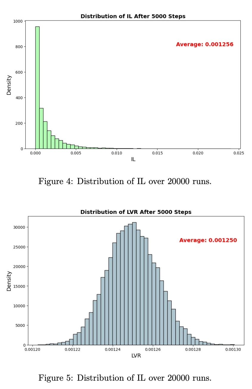
Alexander & Fritz show a deep statistical duality between LVR and IL: LVR is the mathematical expectation of IL.

$$ \mathbb{E}[\text{IL}_T] \approx - \text{LVR}_T $$

• IL is high-variance noise ex post: along any single realized path, IL may be 0 if price mean-reverts, or extremely negative if the market trends one way.
• LVR is deterministic signal ex ante: LVR removes the randomness of price direction and keeps only the cumulative effect of volatility. It is the theoretical expected cost of the LP strategy.

Pricing Logic: The Option Analogy

Since \(LVR \propto \sigma^2 T\), LP losses depend not on predicting price direction but on predicting volatility.
This conclusion leads directly to the key result of Singh et al.: LVR is mathematically equivalent to the funding fee of a perpetual American installment option.

$$ \text{LVR Cost} \equiv \text{Option Premium} $$

This marks a fundamental shift in AMM research. We can directly use implied volatility from mature options markets to price on-chain liquidity positions precisely. In essence, acting as an LP means selling a continuous stream of very short-dated straddles.

Summary and Preview

From a microstructure perspective, the LP in an AMM is not engaging in passive wealth management. The LP is running a short straddle strategy: providing liquidity to the market, collecting fees, and absorbing price-volatility risk in the form of gamma erosion, that is, LVR.

The ultimate formula for judging whether LP provision is profitable is

$$\text{Profit} = \text{Fees} - \text{LVR}$$

• Fees depend on trading activity, that is, noise trading.
• LVR depends on market volatility, specifically on \(\sigma^2\).

Once we understand LVR, we understand why high APY often comes together with high hidden losses. In the next article, AMM Quant Deep Dive 02: The Derivatives Pricing Model of Uniswap V3, we will push this framework further and use option-pricing tools to price and manage Uniswap V3 LP positions more precisely.

---

References

• Alexander, Abe, and Lars Fritz. 2025. “Impermanent Loss and Loss-vs-Rebalancing I: Some Statistical Properties.” arXiv:2410.00854. Preprint, arXiv, May 14. https://doi.org/10.48550/arXiv.2410.00854.
• Cartea, Álvaro, Fayçal Drissi, and Marcello Monga. 2024. “Decentralised Finance and Automated Market Making: Predictable Loss and Optimal Liquidity Provision.” arXiv:2309.08431. Preprint, arXiv, June 13. https://doi.org/10.48550/arXiv.2309.08431.
• Lehar, Alfred, and Christine Parlour. 2025. “Decentralized Exchange: The Uniswap Automated Market Maker.” The Journal of Finance 80 (1): 321–74. https://doi.org/10.1111/jofi.13405.